Information is localized in growing network models
Abstract: Mechanistic network models can capture salient characteristics of empirical networks using a small set of domain-specific, interpretable mechanisms. Yet inference remains challenging because the likelihood is often intractable. We show that, for a broad class of growing network models, information about model parameters is localized in the network, i.e., the likelihood can be expressed in terms of small subgraphs. We take a Bayesian perspective to inference and develop neural density estimators (NDEs) to approximate the posterior distribution of model parameters using graph neural networks (GNNs) with limited receptive size, i.e., the GNN can only "see" small subgraphs. We characterize nine growing network models in terms of their localization and demonstrate that localization predictions agree with NDEs on simulated data. Even for non-localized models, NDEs can infer high-fidelity posteriors matching model-specific inference methods at a fraction of the cost. Our findings establish information localization as a fundamental property of network growth, theoretically justifying the analysis of local subgraphs embedded in larger, unobserved networks and the use of GNNs with limited receptive field for likelihood-free inference.
Paper Prompts
Sign up for free to create and run prompts on this paper using GPT-5.
Top Community Prompts
Explain it Like I'm 14
Overview
This paper studies how to figure out the hidden “settings” (parameters) of rules that grow networks, like social networks or web links, by looking at the final network we can observe. The big idea is that in many realistic models, the important information about these settings is “localized,” meaning it lives in small neighborhoods of the network rather than across the whole thing. This makes the hard problem of inference (guessing the settings from the network) much more manageable.
What questions did the researchers ask?
The researchers wanted to know:
- Do growing network models hide most of their useful information in small parts of the network (local areas)?
- If yes, can we build tools that learn these settings well by only “looking” locally?
- How well do such tools work across different kinds of network-growth rules, especially when the usual math for exact answers is too hard?
How did they study it?
They combined theory and computer experiments.
- Growing networks: Imagine building a network one step at a time. At each step, you pick a “source” node (often a new node) and add connections (edges) to other nodes based on simple rules. Examples: connect to a random person, connect to a friend-of-a-friend, copy some of another node’s links, or add random shortcuts.
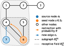
- Localized rules: A rule is called “k-localized” if deciding where to add new edges only depends on the nodes within steps (hops) from a small set of “seed” nodes. A “hop” is like moving from one friend to their friend. If a rule is -localized, the total zone of influence around a source node is its “receptive field,” which is up to $2k+1$ hops wide. Think of it like building a road network where each new road only depends on what’s happening in nearby neighborhoods—not the entire city.
- Why inference is hard: The “likelihood” is a score that says how likely we’d get the observed network if we used certain parameter values. It’s usually too hard to compute exactly because we rarely know the exact order in which edges were added. We typically only see a final snapshot of the network, not its full history.
- Neural tools: They use Neural Density Estimators (NDEs) to learn the “posterior” distribution of parameters (that is, updated beliefs about the parameters after seeing the network). An NDE takes a network as input and outputs a probability distribution over parameters. To read a network, they use Graph Neural Networks (GNNs), which pass messages along edges to compute features. The GNN depth (number of layers) controls how far the network “sees” from each node—like how many hops away it can gather information.
Everyday analogies for key terms: - Inference: Guessing the secret recipe by tasting the cake. - Likelihood: How well a guess for the recipe explains the cake you have. - Posterior (Bayesian): How your belief about the recipe changes after you taste the cake. - GNN: A way for a computer to “read” a network by letting each node talk to its neighbors, then neighbors-of-neighbors, and so on. - Receptive field: How far the GNN can see; more layers mean seeing farther out.
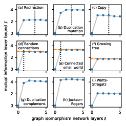
- Experiments: They tested nine different growing network models and trained NDEs on lots of simulated networks. They measured success using a metric related to mutual information (how much the observed network tells you about the parameters). Higher values mean better inference.
What did they find?
- Information is local in many models: For five out of nine models, the rules are localized. For these, the GNN only needs to see a limited neighborhood (up to $2k+1$ hops) to extract nearly all useful information. As they increased the GNN depth, performance rose and then plateaued right when the GNN’s view matched the predicted receptive field size. This matches their theory.
- Works even when not strictly local: For the other models where decisions depend on global structure (not localized), the NDEs still produced high-quality parameter estimates. They often matched specialized, model-specific methods while being much faster.
- Simple models match exact math: For very simple models (like adding random edges), the NDE achieved performance close to exact analytical solutions. This shows the approach is accurate as well as flexible.
- Speed and practicality: Training the NDE takes some time once, but then inference on new networks is extremely fast—under a second—compared to tens of minutes for some traditional methods.
- Limits and improvements: Sometimes deeper GNNs did not help further, either because the task was already saturated at the right locality or because the specific GNN couldn’t capture certain patterns (like triangles). More expressive graph models could help, though they cost more computationally.
Why is this important?
- Makes hard problems doable: The paper shows that in many realistic network-growth scenarios, you don’t need to model the entire network or its hidden history to recover parameters. Focusing on small subgraphs is enough.
- Justifies local analysis: If important information is local, then analyzing small samples of a large network (like neighborhood snapshots) can still be powerful. This is good for privacy and practicality since full, time-stamped data is rare.
- Enables fast, general-purpose tools: Their neural approach provides “off-the-shelf” inference you can apply to many different models without custom derivations. That lets scientists learn from network data quickly and consistently.
Implications and potential impact
- Broader access: Researchers in biology (protein interactions), social science (friend networks), the web, and more can estimate model parameters from snapshots without needing complex, history-aware methods.
- Better privacy and feasibility: Since local subgraphs often suffice, we can infer parameters without collecting sensitive or complete histories.
- Future improvements: Stronger density estimators (like normalizing flows) and more expressive GNNs could push accuracy even higher. Studying how truncated neighborhoods at the edges of samples affect inference will make local methods more robust.
In short, the paper shows that “looking locally” is often all you need to understand how a network grew, and modern neural tools can turn that insight into fast, accurate parameter estimates across many kinds of networks.
Knowledge Gaps
Knowledge Gaps, Limitations, and Open Questions
The following list identifies concrete gaps and unresolved questions that emerge from the paper, targeting areas where future research can act.
- Precise conditions for localization: Formalize necessary and sufficient conditions under which the likelihood of a growing network model can be expressed entirely via small subgraphs (beyond the current assumptions of monotonic growth and seed/source selection independence), including models with structure-dependent seed selection, heterogeneous or time-varying rules, and mixtures of mechanisms.
- Tightness and generality of the receptive field bound: Provide rigorous proofs and potentially tighter bounds for the $2k+1$ receptive field claim, explicitly handling multiple seeds per step, disconnected seed subgraphs, variable across steps, and stochastic exploration processes (e.g., random walks or multi-hop sampling).
- Non-monotonic growth and deletions: Extend the localization framework to models that delete edges or nodes, rewire, or otherwise violate monotonicity (e.g., Watts–Strogatz, duplication–complementation), and determine how receptive fields and localized likelihood expressions should be defined in these settings.
- Directed, weighted, attributed, and multilayer networks: Generalize localization and NDE-based inference to directed edges, weights, node/edge attributes, multiplex/hypergraph structures, and temporal attributes; assess whether local features remain sufficient and what additional local statistics are required.
- Marginal likelihood via local features: Develop algorithmic or theoretical methods to exploit localization for efficient marginalization over unknown source/seed orders (or histories), moving beyond simulation-based inference to scalable approximations that retain local structure.
- Identifiability and model distinguishability: Quantify which parameters and models are formally identifiable from localized subgraph features, especially for models that produce similar local statistics (e.g., duplication–mutation vs copying) or exhibit parameter confounding.
- Posterior fidelity beyond mean-field betas: Evaluate and replace the factorized beta posterior head when posteriors are correlated or multimodal; benchmark normalizing flows or other flexible density estimators against ground-truth posteriors where tractable.
- Calibration and coverage: Assess posterior calibration (e.g., coverage probabilities, posterior predictive checks) and the reliability of uncertainty quantification, not just mutual information, across models and priors.
- Sensitivity to priors and prior misspecification: Analyze how prior choices (e.g., Beta hyperparameters) affect inference quality and mutual information estimates, and develop methods robust to prior misspecification or weak priors.
- Optimization and oversmoothing effects: Diagnose and mitigate performance degradation for deeper GINs (e.g., oversmoothing, vanishing gradients, poor convergence), and test architectural or training remedies (positional encodings, normalization, curriculum learning).
- Higher-order structure extraction: Quantify the impact of missing higher-order features (e.g., triangles, motifs) on parameter recovery; evaluate higher-order GNNs or motif-augmented architectures and the compute–accuracy trade-offs they entail.
- Scaling to large graphs: Establish the computational and statistical scaling of NDEs to networks with millions of nodes/edges; design subgraph-sampling strategies that preserve identifiability and approximation quality for localized inference.
- Partial observations and sampling bias: Study inference from sampled subgraphs (egocentric samples, induced subgraphs, snowball sampling), develop boundary correction for truncated receptive fields, and characterize the bias–variance trade-offs and conditions for consistent estimation.
- Robustness to noise and measurement error: Investigate how missing, spurious, or noisy edges/nodes affect localization and posterior accuracy, and design noise-aware NDEs or likelihood adjustments.
- Time-varying or regime-switching mechanisms: Extend inference to models with changing parameters over time, mixtures of mechanisms, or change points; determine whether localized features can disentangle mechanism mixtures and recover switching dynamics.
- Source/seed selection realism: Relax the assumption of uniform seed/source selection; analyze localization and inference under degree-biased, attribute-biased, or spatially constrained selection and the resulting effect on receptive fields.
- Cross-model generalization and model selection: Test whether a single trained NDE can generalize across related growth mechanisms and support model selection; quantify misclassification rates and propose architectures for joint parameter/model inference.
- Generalization across graph sizes and densities: Verify whether NDEs trained on a fixed node count (e.g., 1,000) generalize to different sizes, densities, and growth horizons; establish size-invariant representations or normalization schemes that preserve identifiability.
- Theoretical reasons for non-localized success: Explain why shallow, limited-receptive-field GNNs recover parameters well for non-localized models (e.g., growing trees), and derive conditions under which global dependencies are effectively captured by local summaries.
- Privacy-preserving localized inference: Explore whether localized features enable privacy-preserving inference (e.g., local subgraph release, differential privacy), and quantify the accuracy/privacy trade-offs and failure modes.
- Evaluation beyond mutual information: Complement mutual information with task-relevant metrics (posterior predictive performance, decision-theoretic utility, out-of-distribution detection), and relate these to localization properties.
- Formal taxonomy of localization: Create a standardized classification of network growth models by localization level (), monotonicity, seed selection mechanism, and neighborhood exploration type, with clear criteria and edge cases.
- Practical guidance for subgraph-only workflows: Provide algorithms and guarantees for inference from only local subgraph samples, including sampling design, boundary correction, and uncertainty propagation when receptive fields are partially observed.
Practical Applications
Immediate Applications
The following items summarize practical uses that can be deployed now, directly leveraging the paper’s findings on information localization in growing networks and the proposed neural density estimator (NDE) workflow.
- Snapshot-based parameter inference for mechanistic network models (Sector: software, social media, web/citation analytics, computational biology)
- Use case: Estimate growth mechanism parameters from a single graph snapshot (e.g., citation networks, web graphs, protein–protein interaction networks) without reconstructing history or full global structure.
- Tool/workflow: A GNN-based NDE service that ingests a graph and returns approximate posteriors for model parameters; mean-pooling and limited-depth GIN as per the paper’s architecture.
- Assumptions/dependencies: Model class is known and appropriate (e.g., monotonic growth, localized mechanisms); prior predictive simulations available; sufficient local subgraphs observed; beta mean-field posterior approximation acceptable.
- Privacy-preserving local inference (Sector: policy, healthcare, social platforms)
- Use case: Analyze growth dynamics (e.g., sexual contact networks, social ties) using only local neighborhoods (ego networks) rather than complete histories, minimizing privacy risks.
- Tool/workflow: Deploy localized GNN inference on subgraph samples; adopt data collection protocols focused on -hop neighborhoods.
- Assumptions/dependencies: Monotonic growth or approximate locality; adequate coverage of receptive fields; potential boundary truncation bias must be quantified.
- Amortized inference for network analysis pipelines (Sector: software, academia)
- Use case: Train NDEs once and reuse to infer parameters on many graphs in under a second, dramatically reducing compute compared to model-specific methods.
- Tool/workflow: Centralized NDE models saved and served via APIs; batch evaluation of new datasets.
- Assumptions/dependencies: Trained on representative synthetic data from the chosen model/prior; monitoring of optimization convergence; careful prior calibration.
- Model selection and plausibility checks across mechanistic models (Sector: academia, research analytics)
- Use case: Compare fit and mutual information across candidate models (e.g., redirection, duplication–mutation, connected small-world) to select mechanisms consistent with observed graphs.
- Tool/workflow: Evaluate NDE-derived posterior fidelity and saturation versus expected receptive field; cross-check against tractable models (e.g., binomial–beta posteriors for 0-localized).
- Assumptions/dependencies: Candidate models cover plausible generative processes; GIN expressivity sufficient for relevant features; avoid overfitting to synthetic training distributions.
- Subgraph-only field studies in public health and social science (Sector: healthcare, social science)
- Use case: Infer contact network growth parameters from sampled local neighborhoods (e.g., clinic or community-level subgraphs) to guide interventions.
- Tool/workflow: Structured -hop sampling and NDE inference; dashboards reporting parameter posteriors and uncertainty.
- Assumptions/dependencies: Sampling strategy avoids systematic bias and covers expected receptive field sizes; monotonic growth approximation holds for the study period.
- Rapid benchmarking and sanity checks for simple models (Sector: academia, education)
- Use case: Validate analytic posteriors (e.g., connected small-world via mean degree, random connection via binomial trials) against NDE outputs to ensure pipeline correctness.
- Tool/workflow: Unit tests using known closed-form posteriors; use mutual information () estimates to assess NDE performance.
- Assumptions/dependencies: Non-degenerate graphs; correct feature extraction (e.g., mean degree from GIN layers); convergence of NDE training.
- Open-source integration for network inference (Sector: software engineering, education)
- Use case: Provide a lightweight reference implementation as a plugin for PyTorch Geometric/Deep Graph Library to enable community adoption in courses and labs.
- Tool/workflow: Reusable NDE modules (GIN + residual MLP + beta head), example notebooks with nine models from the paper.
- Assumptions/dependencies: Availability of synthetic generators and priors; documentation of receptive-field rationale; clear limits for non-localized models.
- Synthetic-data calibration for privacy-preserving releases (Sector: policy, data governance)
- Use case: Fit model parameters to observed networks, then release synthetic networks drawn from calibrated mechanistic models to protect privacy while preserving salient features.
- Tool/workflow: NDE posterior estimation followed by generative resampling under learned parameters; audit of downstream metrics (degree distribution, clustering).
- Assumptions/dependencies: Mechanism adequately captures relevant network properties; synthetic networks meet utility and privacy criteria; regulatory compliance.
Long-Term Applications
The following items outline opportunities that require further research, scaling, or development—particularly extending beyond monotonic/localized growth and improving expressivity and reliability.
- Off-the-shelf network inference engine with a model zoo (Sector: software, cloud platforms)
- Use case: General-purpose platform supporting localized and non-localized models, advanced posteriors (e.g., normalizing flows), and model comparison at scale.
- Tool/workflow: Modular inference APIs; automated prior calibration; streaming ingestion; GPU-accelerated training; mutual information dashboards.
- Assumptions/dependencies: Robust optimization and calibration; support for higher-order features (e.g., triangles); curated library of validated mechanistic models.
- Real-time mechanism monitoring and anomaly detection on large platforms (Sector: social media, web search, cybersecurity)
- Use case: Detect deviations from expected growth (e.g., manipulation, bot amplification) by tracking inferred parameters over time.
- Tool/workflow: Online NDE inference on rolling snapshots; alerting when posteriors shift; integration with trust-and-safety workflows.
- Assumptions/dependencies: Stable data pipelines; partial subgraph sampling sufficiency; calibrated thresholds for alerts; adaptations for non-monotonic events.
- Policy frameworks for local-subgraph data collection (Sector: policy, compliance, healthcare)
- Use case: Codify guidelines that enable scientifically useful inference while limiting sensitive longitudinal data collection.
- Tool/workflow: Standards defining -hop sampling, acceptable truncation, and uncertainty reporting; institutional review board (IRB) templates.
- Assumptions/dependencies: Demonstrated robustness of localized inference under realistic sampling; stakeholder alignment on privacy–utility trade-offs.
- Public health surveillance and intervention planning (Sector: healthcare)
- Use case: Use localized parameter inference on contact networks to estimate mechanisms driving spread or behavior change, informing targeted interventions.
- Tool/workflow: Subgraph-based monitoring in clinics or communities; parameter trajectories linked to policy actions; scenario simulations under inferred mechanisms.
- Assumptions/dependencies: Mechanisms relevant to contagion/contact formation; handling of edge deletion or rewiring; ethical safeguards for sensitive data.
- Financial network risk and AML analytics (Sector: finance)
- Use case: Adapt mechanistic models and localized inference to transaction networks to detect unusual growth patterns and preferential attachment that may indicate risk.
- Tool/workflow: Domain-tailored generators (e.g., account duplication, copying-like behaviors); NDE posteriors feeding compliance scoring tools.
- Assumptions/dependencies: Appropriateness of growth models for financial networks (often non-monotonic with deletions); availability of representative local subgraphs; regulatory alignment.
- Higher-order GNNs and expressive densities for complex structures (Sector: academia, ML research)
- Use case: Capture triangles, motifs, and rich clustering effects to improve inference for non-localized or rewiring models (e.g., Watts–Strogatz).
- Tool/workflow: Extend beyond GIN to higher-order message-passing; replace beta mean-field with normalizing flows; incorporate node attributes.
- Assumptions/dependencies: Increased computational cost; careful regularization; robustness to optimization difficulties and architectural choices.
- Theoretical extensions of localization beyond monotonic growth (Sector: academia)
- Use case: Develop conditions under which information localization holds (or approximately holds) for models with edge deletions/rewiring, and quantify truncation effects rigorously.
- Tool/workflow: New proofs, bounds on receptive fields under non-monotonic dynamics; simulation studies to validate extended theory.
- Assumptions/dependencies: Model classes amenable to analysis; tractable approximations; careful separation of local/global dependencies.
- Active learning for optimal subgraph sampling (Sector: research analytics, policy)
- Use case: Decide which neighborhoods to sample to maximize information about parameters under budget constraints.
- Tool/workflow: Acquisition functions driven by expected mutual information; adaptive sampling protocols; feedback loops with NDE updates.
- Assumptions/dependencies: Reliable uncertainty estimates from NDEs; operational feasibility of targeted sampling; mitigation of sampling bias.
- Robust uncertainty quantification and calibration for decision support (Sector: policy, enterprise analytics)
- Use case: Provide calibrated credible intervals and sensitivity analyses to support policy and business decisions based on inferred mechanisms.
- Tool/workflow: Posterior calibration, prior sensitivity sweeps, conformal prediction overlays; standardized reporting templates.
- Assumptions/dependencies: Well-specified models and priors; consistent convergence behavior; validation on multiple real-world datasets.
- Distributed, large-scale training and evaluation (Sector: cloud computing, enterprise ML)
- Use case: Train NDEs on massive graph corpora and diverse priors, enabling broad transfer and quick deployment across domains.
- Tool/workflow: Distributed simulation and training; dataset versioning; MLOps for model monitoring and updates.
- Assumptions/dependencies: Access to compute resources; scalable synthetic generators; governance over model drift and applicability.
Glossary
- Adam optimizer: A stochastic gradient-based optimization algorithm commonly used to train neural networks. Example: "using the Adam optimizer with an initial learning rate of ~\citep{kingma2017adammethodstochasticoptimization}."
- Amortized inference: An approach that trains a model once to perform fast inference on many instances. Example: "They also provide amortized inference, i.e., the model only needs to be trained once, taking 20~minutes for ."
- Approximate Bayesian computation: A likelihood-free Bayesian method that compares simulated and observed summary statistics to approximate the posterior. Example: "Approximate Bayesian computation draws posterior samples by comparing summary statistics~\cite{Raynal2023},"
- Beta distribution: A probability distribution on [0,1] often used as a prior or posterior for probabilities. Example: "We employ beta distributions because all model parameters are probabilities."
- Bernoulli trials: Independent experiments with two possible outcomes (success/failure) and fixed success probability. Example: "The likelihood is a sequence of Bernoulli trials with success probability ,"
- Bootstrapped 95% confidence intervals: Interval estimates computed via resampling to quantify uncertainty. Example: "Error bars are bootstrapped 95\% confidence intervals and are smaller than markers."
- Clustering coefficient: A measure of the tendency of nodes to form triangles or tightly knit groups. Example: "graphs with short diameter and high clustering coefficients that is easy to study analytically."
- Connected small world model: A small-world network model that adds random edges to a lattice to ensure connectivity. Example: "The connected small world model of \citet{Newman1999} starts with a ring of nodes connected to nearest neighbors, and random connections are added with probability ."
- Duplication-complementation: A network growth mechanism where duplication and selective edge retention or removal mimic functional complementation. Example: "The duplication-complementation~\citep{Vazquez2003}, Jackson-Rogers~\citep{Jackson2007}, and Watts-Strogatz~\citep{Watts1998} models are non-localized variants of the duplication mutation, copying, and connected small world models, respectively."
- Duplication-mutation model: A biological network model where nodes duplicate and edges are retained or mutated with certain probabilities. Example: "\citet{Sole2002} introduced a duplication-mutation model for gene evolution where edges represent physical interactions between expressed proteins."
- Entropy (of the prior): A measure of uncertainty in the prior distribution. Example: "where is the entropy of the prior "
- Expectation-maximization methods: Iterative algorithms for maximum likelihood estimation with latent variables. Example: "approximations include pseudo-marginal likelihood~\citep{Cantwell2021} and expectation-maximization methods~\citep{Larson2023ReversibleNetwork}."
- Gamma function: A continuous extension of the factorial function used in many probability distributions. Example: "where denotes the gamma function."
- Graph isomorphism network (GIN): A message-passing GNN architecture with strong expressive power for graph structure. Example: "First, we use graph isomorphism networks (GINs) with weighted shortcut connections as a local feature extractor."
- Graph neural network (GNN): Neural models that operate on graph-structured data by aggregating information from neighbors. Example: "using graph neural networks (GNNs) with limited receptive size, i.e., the GNN can only ``see'' small subgraphs."
- Heavy-tailed degree distribution: A distribution where high-degree nodes (hubs) occur with significant probability. Example: "such as heavy-tailed degree distributions~\cite{Vazquez2003a},"
- Intractable likelihood: A likelihood function that cannot be computed exactly or efficiently. Example: "Yet inference remains challenging because the likelihood is often intractable."
- Information localization: The property that information about parameters is contained in small local subgraphs rather than the whole network. Example: "Our findings establish information localization as a fundamental property of network growth,"
- Jackson-Rogers model: A social network growth model where nodes connect via random and friends-of-friends mechanisms. Example: "Jackson-Rogers~\citep{Jackson2007}"
- k-hop neighborhood: The set of nodes within k steps (edges) from a given node. Example: "induced by the -hop neighborhoods of seeds in ."
- k-localized: Describes models where new edges depend only on subgraphs within k hops of certain seeds. Example: "We say that a rule is -localized if new edges only depend on the subgraphs $B_{S_{t}^{(k)}{G_{t-1}$"
- Likelihood-free inference: Inference methods that do not evaluate the likelihood explicitly, often using simulations. Example: "the use of GNNs with limited receptive field for likelihood-free inference."
- Mean-field approximation: A variational assumption that the posterior factorizes into independent components. Example: "This parametric approximation assumes that the posterior factorizes similar to a variational mean-field approximation."
- Mean-pooling: Aggregating node features by averaging to obtain a graph-level representation. Example: "After applying the GIN times, we mean-pool node features to obtain the graph-level representation "
- Mechanistic network model: A model based on interpretable rules that generate networks reflecting real-world mechanisms. Example: "Mechanistic network models can capture salient characteristics of empirical networks using a small set of domain-specific, interpretable mechanisms."
- Message-passing graph neural networks: GNNs that iteratively aggregate information from neighbors to update node embeddings. Example: "While GINs are provably the most expressive message-passing graph neural networks~\citep{Xu2019a},"
- Monotonic growth: A growth process where edges are never deleted as the network evolves. Example: "We assume that edges are never deleted, and we call the growth monotonic."
- Mutual information: A measure of the information shared between parameters and observations. Example: "for the mutual information between parameters and graph observations,"
- Neural density estimator (NDE): A neural model that estimates a probability density (e.g., posterior) from data. Example: "we resort to simulation-based inference using neural density estimators (NDEs) \cite{Papamakarios2016epsilon-free}."
- Normalizing flows: Flexible density estimators that transform simple distributions into complex ones via invertible mappings. Example: "such as normalizing flows~\cite{Papamakarios2021}."
- Posterior distribution: The probability distribution over parameters given observed data. Example: "develop neural density estimators (NDEs) to approximate the posterior distribution of model parameters"
- Preferential attachment: A mechanism where nodes with higher degree attract new connections more likely. Example: "When , the model is equivalent to preferential attachment~\cite{Barabasi1999}."
- Prior predictive distribution: The distribution of data simulated from the prior through the generative model. Example: "where denotes the expectation under the prior predictive distribution~\citep{Papamakarios2016epsilon-free}."
- Probabilistic redirection model: A growth model where new edges occasionally redirect to neighbors of a randomly chosen seed. Example: "Illustration of network growth for a probabilistic redirection model~\cite{Krapivsky2001.}"
- Pseudo-marginal likelihood: An approach that uses unbiased likelihood estimates within likelihood-based inference. Example: "approximations include pseudo-marginal likelihood~\citep{Cantwell2021}"
- Receptive field: The subgraph region that can influence or be influenced by a node’s creation step in the model. Example: "we call the subgraph the receptive field of node ."
- Residual connections: Network connections that add inputs to outputs of layers to stabilize training. Example: "Second, we apply dense residual layers with the same functional form as the GIN layer MLPs"
- Simulation-based inference: Inference using simulations of the generative model instead of explicit likelihoods. Example: "we resort to simulation-based inference using neural density estimators (NDEs)"
- Small-world effect: The phenomenon of short average path lengths and high clustering in networks. Example: "the small-world effect~\cite{Watts1998},"
- Softplus activation function: A smooth approximation of ReLU defined as log(1+exp(x)). Example: "softplus activation function "
- Sufficient statistic: A function of the data that captures all information needed to determine the posterior for a parameter. Example: "which is a sufficient statistic that fully determines the posterior"
- Variational lower bound: A lower bound on a quantity (e.g., mutual information) expressed via variational approximations. Example: "We evaluated NDEs by estimating a variational lower bound "
- Variational mutual information: An estimate of mutual information computed via a variational objective. Example: "Each panel shows an estimate of the variational mutual information as a function of GIN depth ,"
- Watts-Strogatz model: A network model that rewires edges in a ring lattice to interpolate between regular and random graphs. Example: "\subsection{\modelnumref.\ Watts-Strogatz model}"
- Weighted shortcut connections: Scaling residual (skip) connections to stabilize gradients in deep GNNs. Example: "First, we use graph isomorphism networks (GINs) with weighted shortcut connections as a local feature extractor."
Collections
Sign up for free to add this paper to one or more collections.