A Proof of Learning Rate Transfer under $μ$P
Abstract: We provide the first proof of learning rate transfer with width in a linear multi-layer perceptron (MLP) parametrized with $\mu$P, a neural network parameterization designed to ``maximize'' feature learning in the infinite-width limit. We show that under $\mu P$, the optimal learning rate converges to a \emph{non-zero constant} as width goes to infinity, providing a theoretical explanation to learning rate transfer. In contrast, we show that this property fails to hold under alternative parametrizations such as Standard Parametrization (SP) and Neural Tangent Parametrization (NTP). We provide intuitive proofs and support the theoretical findings with extensive empirical results.
Paper Prompts
Sign up for free to create and run prompts on this paper using GPT-5.
Top Community Prompts
Explain it Like I'm 14
Overview
This paper studies a simple but important question in training neural networks: how should we choose the learning rate when we make a network wider? The authors prove that, under a specific way of setting up a network called μP (Maximal Update Parametrization), the best learning rate stays roughly the same even as the network gets very wide. This is called “learning rate transfer.” They also show that this helpful property does not hold under other common setups.
Key Objectives
The paper focuses on three main goals:
- Explain, with a proof, why the best learning rate doesn’t need to change as we make a network wider if we use μP.
- Show that this “learning rate transfer” fails under other ways of setting up neural networks (like the Standard Parametrization, SP, and Neural Tangent Parametrization, NTP).
- Support the theory with experiments on different network sizes, depths, and training setups.
Methods and Approach
Think of a neural network as a machine with layers that transform inputs into outputs. Two important ideas here:
- Width: how many “units” each layer has. Making the network wider means adding more units per layer.
- Learning rate: a knob that controls how big each training step is. If it’s too big, training can explode; if it’s too small, training is slow or stalls.
What the authors did:
- They studied a simple kind of network called a “linear MLP.” It has multiple layers, but no activation functions like ReLU. This makes math cleaner.
- They showed that, after one training step, the network’s loss (how wrong it is) can be written as a polynomial in the learning rate. A polynomial is just a sum like a×(LR) + b×(LR)2 + c×(LR)3, and so on.
- Under μP, most of the higher powers of the learning rate fade away as the network gets very wide, leaving a simple curve with a clear best learning rate that doesn’t go to zero.
- They then extended the idea to more training steps. The math gets more complicated (more terms matter), but the key trick remains: analyze how those polynomial terms behave as width grows.
- They used standard probability results to show the coefficients of those polynomials settle to fixed values when the network gets very wide, which pins down a stable best learning rate.
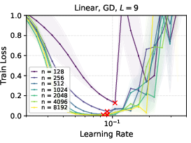
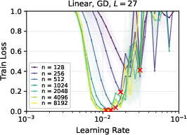
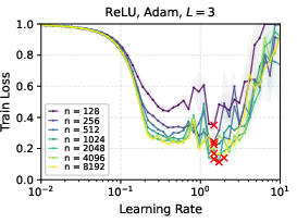
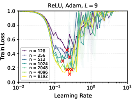
- Finally, they ran lots of experiments to confirm their proofs. They checked linear networks trained with gradient descent, and also tried ReLU networks and Adam optimizers to see how well the idea holds up in practice.
To make the technical terms friendlier:
- μP (Maximal Update Parametrization): a careful way to set the scale of the network’s weights and learning rate so that the network’s “features” (the internal patterns it learns) keep changing meaningfully even when the network is very wide.
- SP (Standard Parametrization): the usual default setup many libraries use. It doesn’t guarantee stable behavior as you make the network wider.
- NTP (Neural Tangent Parametrization): a setup that makes extremely wide networks behave like fixed kernels (their features barely change). That often means you need a very different learning rate behavior.
Main Findings
Here are the most important results:
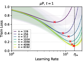
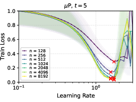
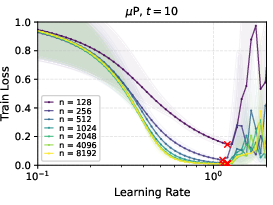
- Under μP, the best learning rate converges to a non-zero constant as the network width grows. Translation: you can tune the learning rate on a smaller, narrower network and reuse it for much wider versions.
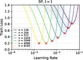
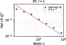
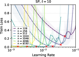
- Under SP, the best learning rate shrinks toward zero as you make the network wider. So you would need to keep retuning it, which is costly and inconvenient.
- Under NTP, the needed learning rate tends to blow up as the network gets wider, which is also bad for easy tuning.
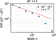
- They proved this carefully after one training step and showed the convergence rate is fast (roughly like 1 divided by the square root of the width), and then extended the proof idea to multiple training steps.
- Experiments matched the theory:
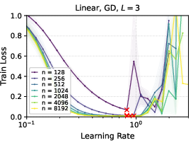
- In linear networks trained with gradient descent, μP showed clean learning rate transfer; SP did not.
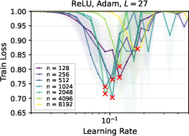
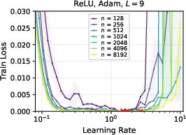
- With ReLU networks and Adam optimizer, μP still showed strong learning rate transfer in practice, even though the formal proof was for linear networks.
- Deeper networks tend to prefer smaller learning rates, but the “transfer” property still holds under μP.
- Later in training, the range of “good enough” learning rates widens, making it less sensitive to the exact value.
Implications and Impact
This research provides a solid mathematical reason to trust learning rate transfer under μP. That’s a big deal because:
- It saves time and money: you can tune your learning rate once on a smaller model and reuse it on larger ones.
- It reduces guesswork and instability when scaling models.
- It helps bridge the gap between theory and practice: we now know when and why learning rate transfer should happen.
Limitations and future directions:
- The formal proofs cover linear networks trained with gradient descent. The experiments suggest similar behavior in more realistic setups (ReLU and Adam), but full proofs there are future work.
- The result depends on mild assumptions (like there being a clear best learning rate at each step), which usually hold in practice.
In short: if you set up your network using μP, the best learning rate doesn’t drift as you make it wider. You can tune once and reuse—making scaling smoother and more reliable.
Knowledge Gaps
Knowledge gaps, limitations, and open questions
Below is a concise list of what remains missing, uncertain, or unexplored in the paper, framed to enable concrete follow-up research.
- Extension beyond linear MLPs: The proofs are restricted to deep linear networks with GD and quadratic loss. A rigorous theory for non-linear activations (e.g., ReLU), modern losses (e.g., cross-entropy), and non-linear feature dynamics is not provided.
- Optimizer generality: Learning rate (LR) transfer is only proved for full-batch gradient descent. The behavior under common optimizers (SGD with momentum, Adam with scaling, Adagrad, RMSProp) and their width-dependent preconditioning remains theoretically unresolved.
- Stochastic training: The impact of gradient noise (mini-batching), batch size scaling, and stochastic optimization on LR transfer and its asymptotics is not analyzed.
- Training deeper “input/output” layers: The theory fixes and . A formal analysis when and are trainable (including the specified P LR scaling for ) is missing, as is the effect of training these layers on LR transfer.
- Multi-output networks: Although the text states results “can be generalized” to multi-dimensional outputs, no explicit proof or scaling rules (especially for ) are given for multi-output architectures.
- General-step characterization: For , LR transfer is shown to exist but without:
- An explicit expression for the limiting optimal LR (analogous to the closed-form at ).
- Non-asymptotic or asymptotic convergence rates for .
- Conditions guaranteeing convexity/uniqueness of the limiting minimizer for general (the uniqueness assumption is taken as “mild” but unproven/generic).
- Convergence-rate anomaly: Empirically at , the observed rate changes abruptly beyond , deviating from the prediction. The cause of this regime shift and whether tighter (or different) rates hold asymptotically is left unexplained.
- Assumption sensitivity: The results rely on Gaussian i.i.d. initialization and independence assumptions in Tensor Programs. Robustness to:
- Non-Gaussian initializations (e.g., orthogonal, truncated, heavy-tailed).
- Architectural inductive biases (e.g., weight sharing in CNNs, residual connections).
- Bias parameters and normalization layers (BatchNorm, LayerNorm).
- is not studied.
- Dataset structure: The assumption is crucial but its failure modes are not characterized. What happens when (near-degenerate Gram–label alignment), or when has poor conditioning?
- Depth scaling: While experiments vary depth, the theory does not treat depth-to-infinity regimes or Depth-P. Formal depth-scaling exponents and their effect on LR transfer (including potential joint width–depth limits) remain open.
- Alternative parameterizations: For SP/NTP, only qualitative failure modes are provided. A full characterization of optimal LR scaling (e.g., can SP regain LR transfer with LR ∝ or another exponent?) is not analyzed.
- Finite-width corrections: No non-asymptotic bounds quantify how large must be for practical LR transfer, or provide finite- error terms between and beyond .
- Generalization vs. training loss: The results focus on training loss. Whether LR transfer under P correlates with generalization performance, stability, and edge-of-stability phenomena (and how these differ across parameterizations) is not investigated.
- Loss landscapes and multimodality: For , the limiting polynomial could, in principle, have multiple minima depending on data and initialization. A rigorous analysis of when uniqueness holds and how to detect/handle multimodality is lacking.
- Real-data validation: Experiments use synthetic data. Whether the theoretical predictions and LR transfer properties hold across real datasets and architectures (CNNs, Transformers) remains empirically and theoretically open.
- LR schedules: The analysis covers constant LR only. The interaction of width scaling with practical LR schedules (warmup, cosine decay, step decay) and their transferability is unaddressed.
- Regularization: The effects of explicit regularizers (weight decay, dropout), implicit bias from optimization, and their scaling under P on LR transfer are unknown.
- Classification settings: The theory uses quadratic loss; LR transfer under standard classification losses (e.g., logistic/cross-entropy) is not proved.
- Polynomial structure at higher steps: Beyond , the degree and coefficient structure of the limiting polynomials are not characterized, making it hard to derive analytic properties (e.g., convexity, minimizer location, sensitivity) at general .
- Quantifying failure under NTP: While LR under NTP is argued to blow up, a formal width-dependent rate of divergence and its implications for practical tuning are not derived.
- Multi-step dynamics and interaction terms: The proofs do not track how cross-terms across steps (e.g., dependence of , , and on ) shape the limiting loss landscape, leaving open a systematic way to compute or bound these higher-order contributions.
- Robustness to noisy labels and misspecification: Sensitivity of LR transfer to label noise, model misspecification, and non-linear ground truth (beyond the empirical ReLU case) lacks theoretical treatment.
- Scaling with sample size and dimension: How LR transfer depends on and (beyond the Gram dependence at ), including high-dimensional asymptotics and conditioning of , is not analyzed.
- Practical tuning guidance: The paper shows existence and convergence but does not translate the asymptotic theory into actionable finite-width tuning rules (e.g., recommended base width, LR search ranges, depth-dependent scaling constants).
Practical Applications
Immediate Applications
The following applications can be deployed now, leveraging the paper’s theoretical guarantees for linear networks and its empirical evidence for ReLU MLPs and common optimizers.
- Hyperparameter tuning cost reduction in ML pipelines (software/MLOps)
- Use case: Tune learning rate (LR) on a small-width model under μP, then reuse the same LR for larger-width models without re-tuning.
- Workflow: Adopt μP initialization and LR scaling (GD: constant LR; Adam: LR ∝ n⁻¹). Tune LR at width n₀ (e.g., 2¹⁰), validate transfer at larger widths (e.g., 2¹⁴–2¹⁶).
- Tools: μP-aware wrappers for PyTorch/TensorFlow layers; AutoML integration for “tune-small, deploy-big.”
- Assumptions/dependencies: Requires μP parameterization (not SP/NTP); projection layer V variance ∝ n⁻²; training with GD/SGD/Adam; non-degenerate input Gram matrix (Ky ≠ 0); unique minimizer of the limiting loss.
- Faster experimentation and reproducibility in academia (academia/software)
- Use case: Standardize experimental setups with μP so learning rate settings remain stable across width, improving reproducibility in scaling studies.
- Workflow: Report LR settings alongside μP initialization rules; run ablations at small widths to infer LRs for larger widths.
- Tools: Experimental protocol checklists; μP “recipe cards” for linear and ReLU MLPs; notebooks that verify LR transfer via convergence plots.
- Assumptions/dependencies: Applicability is strongest for linear MLPs (proven), with empirical support for ReLU+Adam; caution with more complex architectures.
- Energy and cost savings for model training (energy/finance/software)
- Use case: Reduce hyperparameter sweeps that scale poorly with width, lowering cloud/HPC costs and energy consumption.
- Workflow: Limit LR sweeps to small widths; apply learned LR to larger widths; monitor training stability (loss vs. LR).
- Tools: Training cost dashboards; LR transfer monitors; CI/CD hooks to gate large-width runs until LR is validated.
- Assumptions/dependencies: Savings depend on eliminating width-dependent LR retuning; broader savings scale with how often width is increased.
- Practical guidance for model scaling in product teams (software/consumer tech)
- Use case: Teams scaling feed-forward or simple ReLU MLPs for recommendation, ranking, or tabular prediction can adopt μP to stabilize LR across width.
- Workflow: Convert SP to μP by changing V initialization variance to n⁻²; adopt width-aware LR choice; implement guardrails to avoid SP/NTP defaults.
- Tools: μP migration guides; linters that flag non-μP parameterization; “μP presets” in framework configs.
- Assumptions/dependencies: Most effective for architectures close to those tested (MLPs); SP/NTP defaults in popular frameworks may need overriding.
- AutoML and hyperparameter search enhancements (software)
- Use case: Shrink the search space for LR in width-scaling experiments; bias search toward μP-consistent LRs.
- Workflow: Two-stage search: (1) small-width LR tuning; (2) width scaling with fixed LR. Optionally refine LR in a narrow band near the theoretical optimum.
- Tools: AutoML plugins that enforce μP scaling and carry LRs forward across widths; Bayesian optimization seeded with μP priors.
- Assumptions/dependencies: Requires compact LR intervals for optimization; relies on convergence rates (often O(n⁻¹/²)) for practical widths.
- Curriculum and lab design for scaling behaviors (education)
- Use case: Teach students scaling laws and parameterizations via μP, demonstrating LR transfer vs. failure under SP/NTP.
- Workflow: Labs comparing train loss vs. LR at different widths; measure convergence of the optimal LR; discuss Gram matrix role and depth effects.
- Tools: Course modules; interactive visualizations of LR transfer; exercises replicating figures similar to the paper’s setups.
- Assumptions/dependencies: Students should have basics in initialization, optimization, and large-width limits.
- Benchmarking and diagnostics for LR sensitivity (software/quality assurance)
- Use case: Establish LR transfer diagnostics to catch width-induced LR drift in SP/NTP pipelines.
- Workflow: Plot loss vs. LR across widths; flag cases where the optimal LR shifts toward zero (SP) or diverges (NTP).
- Tools: “LR transfer score” metrics; automated reports in training logs; comparison harnesses between μP and SP/NTP.
- Assumptions/dependencies: Diagnostic thresholds calibrated on known convergence rates; uses compact LR intervals.
Long-Term Applications
These applications require further research and engineering, particularly to generalize proofs beyond linear networks and integrate into complex production systems.
- Standardization of μP-like parameterizations across frameworks (software/standards)
- Use case: Make μP default or available as a first-class option in PyTorch/TensorFlow/JAX for MLPs/CNNs/Transformers.
- Workflow: Develop library-level parameterization APIs; certify “μP-compliant” initializations and optimizer scalings; include Depth-μP variants.
- Tools: μP core libraries; compliance tests; reference implementations for common architectures.
- Assumptions/dependencies: Proofs for nonlinear and attention-based architectures; compatibility with mixed-precision and distributed training.
- μP-aware optimizers and schedules (software/optimization research)
- Use case: Design optimizers or LR schedules that exploit polynomial-in-η loss structure and μP transfer properties.
- Workflow: Derive adaptive schedules from early-step polynomial approximation; create μP-aware Adam variants; integrate with “edge of stability” insights.
- Tools: Optimizer plugins; LR schedule generators; training telemetry that estimates polynomial coefficients online.
- Assumptions/dependencies: Robust estimation of coefficients in non-linear regimes; guarantees for complex architectures.
- Scaling laws and governance for green AI (policy/energy/academia)
- Use case: Reduce hyperparameter sweep emissions by institutionalizing μP-based “tune-small” standards in grants, benchmarks, and procurement.
- Workflow: Policies requiring documented use of LR transfer methods; carbon budgets that penalize width-dependent retuning.
- Tools: Reporting templates; audit tools tracking tuning runs; benchmark guidelines rewarding μP-based efficiency.
- Assumptions/dependencies: Broad acceptance of μP; metrics linking μP adoption to measurable energy savings.
- Federated and on-device scaling strategies (software/edge/robotics)
- Use case: Transfer LRs from compact on-device models to larger server models, or from simulation to higher-capacity real robots.
- Workflow: μP-tuned LR at small width on-device/in-simulation; scale width for server-side or production hardware without re-tuning LR.
- Tools: Federated training orchestration with μP parameterization; simulators using μP-aware model scaling.
- Assumptions/dependencies: Extension of LR transfer to architectures used on edge/robots; constraints from heterogeneous hardware.
- Sector-specific adoption in high-stakes domains (healthcare/finance)
- Use case: Accelerate model iteration by stabilizing LR across width when scaling tabular/MLP models for risk scoring or imaging.
- Workflow: Validate μP LR transfer on domain datasets; incorporate μP into risk management pipelines and clinical ML development.
- Tools: Compliance-ready μP training recipes; LR transfer validation reports for audits; domain-specific AutoML with μP.
- Assumptions/dependencies: Clinical/financial models may use architectures beyond linear/MLP; regulatory acceptance requires rigorous validation.
- μP-based training autopilots and dashboards (software/MLOps)
- Use case: End-to-end systems that tune at small width, predict LR transfer, orchestrate scaling, and monitor deviations.
- Workflow: Implement “HP Transfer Toolkit” that handles initialization, LR tuning, scaling plans, and alerting on transfer failures.
- Tools: Orchestration engines; LR transfer monitors; width-scaling simulators; integration with Ray/Tune, Kubernetes, and major DL frameworks.
- Assumptions/dependencies: Reliable transfer across architectures; strong telemetry to detect exceptions and re-tune only when necessary.
- Deeper theoretical generalization and guarantees (academia)
- Use case: Extend proofs to non-linear networks (CNNs, Transformers), residual connections, and modern training tricks (weight decay, normalization).
- Workflow: Combine Tensor Programs with mean-field and NTK/feature-learning analyses; formalize conditions for unique minimizers and convergence rates.
- Tools: Theoretical toolkits; synthetic benchmarks designed to map boundaries of LR transfer.
- Assumptions/dependencies: Mathematical tractability, particularly for attention/residual dynamics; careful control of large-width deviations.
Key Assumptions and Dependencies
- μP parameterization is correctly implemented:
- Initialization: W₀ ∼ N(0, d⁻¹), Wₗ ∼ N(0, n⁻¹), V ∼ N(0, n⁻²).
- Learning rate: GD uses constant LR; Adam uses LR ∝ n⁻¹ (c = 1).
- Dataset and geometry:
- Input Gram matrix non-degenerate (Ky ≠ 0).
- Loss landscape with a unique minimizer at each step t.
- Proven scope vs. empirical scope:
- Theoretical guarantees for linear MLPs with GD (and detailed one-step convergence at O(n⁻¹/²)).
- Empirical support for ReLU MLPs and Adam; mixed results reported in LLM literature.
- Framework defaults:
- SP/NTP defaults in common libraries can break LR transfer (optimal LR shifts to zero or diverges); must override to μP.
Glossary
- Adam: An adaptive gradient-based optimizer that uses estimates of first and second moments of gradients to adjust learning rates per parameter. "For the learning rate, μP scaling parametrizes the learning rate as η n{-1} for Adam [yang2022tensor] and η for gradient descent."
- Almost sure convergence: A strong form of convergence of random variables where the sequence converges with probability 1. "As n→∞, all the coefficients converge almost surely to deterministic constants."
- Argmin: The set or value of the argument that minimizes a function. "Given width n and training step t, an optimal LR can be defined as η{n}{(t)} ∈ \textrm{argmin}{\eta > 0} L_n{(t)}(\eta)."
- Bayesian neural network: A neural network with probabilistic weights, treating weights as random variables with specified priors. "Neal1996 was the first to introduce the “1/\textrm{fan-in}” initialization in the context of Bayesian neural networks."
- Big-O notation: Asymptotic notation that describes an upper bound on the growth rate of a function. "we write c_n = O(d_n) when c_n < \kappa d_n for n large enough, for some constant \kappa > 0."
- Convergence in probability: A mode of convergence where random variables get arbitrarily close to a constant with high probability as the sample size grows. "We say that LR transfers with width n if there exists a deterministic constant η\infty{(t)}> 0 such that the optimal learning rate η_n{(t)} converges in probability to a η\infty{(t)} as n goes to infinity."
- Edge of stability: A regime in training where the learning rate is close to the threshold that destabilizes gradient descent dynamics. "Learning rate transfer was empirically studied in \cite{noci2024superconsistencyneuralnetwork} from the angle of Hessian geometry (and its connection to the edge of stability \cite{cohen2022gradientdescentneuralnetworks})"
- Fan-in: The number of input connections to a neuron; used to scale initialization to maintain activation magnitudes. "He initialization \citep{he2016deep} introduced the “1/\textrm{fan-in}” initialization which normalizes the weights to achieve order one activations as width grows"
- Feature learning: The process by which a network modifies internal representations (features) during training, rather than behaving like a fixed kernel. "The authors showed that under the neural tangent parametrization, training dynamics converge to a kernel regime in the infinite-width limit, a phenomenon known as lazy training ... which exhibit significant feature learning."
- Gaussian process: A stochastic process where any finite set of points has a joint Gaussian distribution; emerges as a limit of certain wide networks. "showed that single-layer Bayesian networks converge to a Gaussian process in the infinite-width limit"
- Gram matrix: A matrix of inner products between vectors, often used to analyze data geometry. "we define the m\times m normalized input Gram matrix K=\left(d{-1}\,\langle x_i,x_j\rangle\right)_{1\leq i,j \leq m} \in\mathbb R{m\times m}"
- He initialization: A weight initialization scheme scaling by 1/fan-in to stabilize activations and gradients in deep networks. "He initialization \citep{he2016deep} sets the initialization weights as centred gaussian random variables with “1/fan_in” variance"
- Hessian geometry: Geometric properties derived from the Hessian (second derivative) of the loss, used to understand optimization behavior. "from the angle of Hessian geometry (and its connection to the edge of stability \cite{cohen2022gradientdescentneuralnetworks})"
- Hyperparameter (HP) transfer: The phenomenon where optimal hyperparameters remain stable across model scales, enabling reuse without retuning. "A nice by-product of μP is HP transfer, or where optimal HPs seem to converge as width increases"
- Infinite-width limit: The theoretical regime where the number of neurons per layer tends to infinity, revealing simplified training dynamics. "a neural network parameterization designed to “maximize” feature learning in the infinite-width limit."
- Kernel regime: A training regime where the network behaves like a fixed kernel method, with features not changing significantly. "training dynamics converge to a kernel regime in the infinite-width limit"
- Lazy training: A regime where network features stay close to their initialization and training is approximately linear around that point. "a phenomenon known as lazy training \citep{chizat2020lazytrainingdifferentiableprogramming}"
- Learning rate (LR) transfer: Stability of the optimal learning rate as model width increases, allowing reuse across scales. "We provide the first proof of learning rate transfer with width in a linear multi-layer perceptron (MLP) parametrized with μP"
- L2 norm: The Euclidean norm; also used to define convergence in second moment for random variables. "asymptotics are defined in the sense of the second moment ( norm)."
- Maximal Update Parametrization (μP): A parameterization that sets scaling exponents to maximize feature learning and enable hyperparameter transfer. "introduced the Maximal Update Parametrization (P) which sets precise scaling exponents for the initialization and learning rate."
- Mean-field initialization: An initialization scaling motivated by mean-field theory, often leading to nontrivial limits as width grows. "the convergence of to $0$ is a result of the fact that converges to zero because of the Mean-field-type initialization of the projection layer ."
- Mean-field neural networks: A theoretical framework analyzing networks via mean-field limits and partial differential equations. "and the literature on mean-field neural networks \citep{sirignano2019meanfieldanalysisneural, mei2019meanfieldtheorytwolayersneural, Mignacco_2021, chizat2022infinitewidthlimitdeeplinear}"
- Multi-Layer Perceptron (MLP): A feedforward neural network with multiple layers of linear transformations (and optionally nonlinearities). "We consider a linear Multi-Layer Perceptron (MLP) given by f(x) = V\top W_L W_{L-1} \dots W_1 W_0 x"
- Neural parametrization: A specification of how initialization and learning rate scale with width and depth. "A neural parametrization for model \cref{eq:mlp} specifies the constants , and "
- Neural Tangent Kernel (NTK): A kernel that describes training dynamics of infinitely wide networks under certain parameterizations. "The Neural Tangent Kernel (NTK, \citep{jacot2018neural}) was one of the first attempts to understand training dynamics of large-width neural networks."
- Neural Tangent Parametrization (NTP): A parameterization in which training dynamics converge to the NTK kernel regime. "In contrast, we show that this property fails to hold under alternative parametrizations such as Standard Parametrization (SP) and Neural Tangent Parametrization (NTP)."
- Outer product: The product of two vectors producing a matrix, used in expressing rank-1 updates. "For two vectors , denotes the outer product."
- Projection layer: The final layer vector/matrix mapping hidden activations to outputs; denoted by V in the model. "the Mean-field-type initialization of the projection layer ."
- Rank-1 matrix: A matrix that can be expressed as the outer product of two vectors; appears in gradient expressions. "the gradients are given by rank-1 matrices"
- ReLU: A nonlinear activation function defined as max(0, x), commonly used in deep networks. "MLP with ReLU activation of varying depth trained with Adam."
- Standard Parametrization (SP): A common parameterization (e.g., PyTorch defaults) without width-dependent learning rate scaling. "Standard Parametrization (SP): for , , and ."
- Strong Law of Large Numbers (SLLN): A theorem ensuring sample averages converge almost surely to expected values. "Strong Law of Large Numbers (SLLN) as yields convergence to almost surely."
- Tensor Programs: A framework for analyzing wide-network limits via program-like derivations and master theorems. "The convergence of the coefficients to deterministic limit follows from the “Master Theorem” in \cite{yang2021tensor}."
- Uniform convergence on compact sets: Convergence of functions such that the maximum deviation over any compact domain tends to zero. "The -step loss converges almost surely to uniformly over on any compact set."
Collections
Sign up for free to add this paper to one or more collections.