Learning Sparse Approximate Inverse Preconditioners for Conjugate Gradient Solvers on GPUs
Abstract: The conjugate gradient solver (CG) is a prevalent method for solving symmetric and positive definite linear systems Ax=b, where effective preconditioners are crucial for fast convergence. Traditional preconditioners rely on prescribed algorithms to offer rigorous theoretical guarantees, while limiting their ability to exploit optimization from data. Existing learning-based methods often utilize Graph Neural Networks (GNNs) to improve the performance and speed up the construction. However, their reliance on incomplete factorization leads to significant challenges: the associated triangular solve hinders GPU parallelization in practice, and introduces long-range dependencies which are difficult for GNNs to model. To address these issues, we propose a learning-based method to generate GPU-friendly preconditioners, particularly using GNNs to construct Sparse Approximate Inverse (SPAI) preconditioners, which avoids triangular solves and requires only two matrix-vector products at each CG step. The locality of matrix-vector product is compatible with the local propagation mechanism of GNNs. The flexibility of GNNs also allows our approach to be applied in a wide range of scenarios. Furthermore, we introduce a statistics-based scale-invariant loss function. Its design matches CG's property that the convergence rate depends on the condition number, rather than the absolute scale of A, leading to improved performance of the learned preconditioner. Evaluations on three PDE-derived datasets and one synthetic dataset demonstrate that our method outperforms standard preconditioners (Diagonal, IC, and traditional SPAI) and previous learning-based preconditioners on GPUs. We reduce solution time on GPUs by 40%-53% (68%-113% faster), along with better condition numbers and superior generalization performance. Source code available at https://github.com/Adversarr/LearningSparsePreconditioner4GPU
Paper Prompts
Sign up for free to create and run prompts on this paper using GPT-5.
Top Community Prompts
Explain it Like I'm 14
What is this paper about?
This paper is about making a popular math tool called the Conjugate Gradient (CG) solver run faster on graphics cards (GPUs). CG is used to solve huge systems of equations that show up in physics, engineering, and simulations (like heat flow or how materials bend). To make CG fast, you usually add a “helper” called a preconditioner. This paper teaches a neural network to build a new kind of helper that runs extremely well on GPUs and speeds up the solver a lot.
What questions are the researchers asking?
They focus on three clear questions:
- Can we design a preconditioner that works well with GPUs (which are best at doing many small tasks at once)?
- Can we use a Graph Neural Network (GNN) to learn this preconditioner from data, so it adapts to many types of problems?
- Can we train it with a smart “loss function” that measures progress in a way that matches what CG actually cares about (so it learns faster and better)?
How did they do it?
Think of solving equations like finding the quickest path through a maze. The CG solver moves step by step toward the exit. A preconditioner reshapes the maze to make straight paths easier to find.
- The problem with some traditional helpers (like Incomplete Cholesky, IC) is that they involve “triangular solves.” That’s like having to climb a ladder one rung at a time—you can’t parallelize it well. GPUs prefer doing thousands of small, independent tasks at once, not ladder-climbing.
- The authors choose a different helper: a Sparse Approximate Inverse (SPAI). Instead of factoring the matrix (ladder), SPAI tries to build a lightweight “cheat sheet” that directly approximates the inverse. Using this cheat sheet during CG boils down to just two sparse matrix–vector multiplications per step—perfect for GPUs.
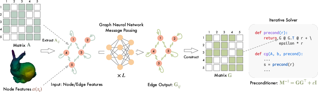
- They use a Graph Neural Network to build that cheat sheet. A matrix can be viewed as a graph: each variable is a node, and a nonzero connection between variables is an edge. GNNs naturally pass information along edges in small neighborhoods, which matches how SPAI operates (it mostly needs local information). The GNN outputs a sparse matrix G, and the preconditioner is built as M⁻¹ = G Gᵀ + a tiny safety term to keep it well-behaved.
- Training trick: They introduce a new loss called SAI (Scale-invariant Aligned Identity). CG’s speed depends on the “shape” of the problem (its condition number), not the overall size of the numbers. The SAI loss measures how close A * M⁻¹ is to the identity matrix, but it normalizes out the scale first—like adjusting the volume knob before comparing songs. They also use random probe vectors to estimate this efficiently without solving big systems during training.
In short: they treat the matrix as a graph, use a GNN to produce a GPU-friendly preconditioner (SPAI), and train it with a scale-aware loss that matches what matters for CG.
What did they find, and why is it important?
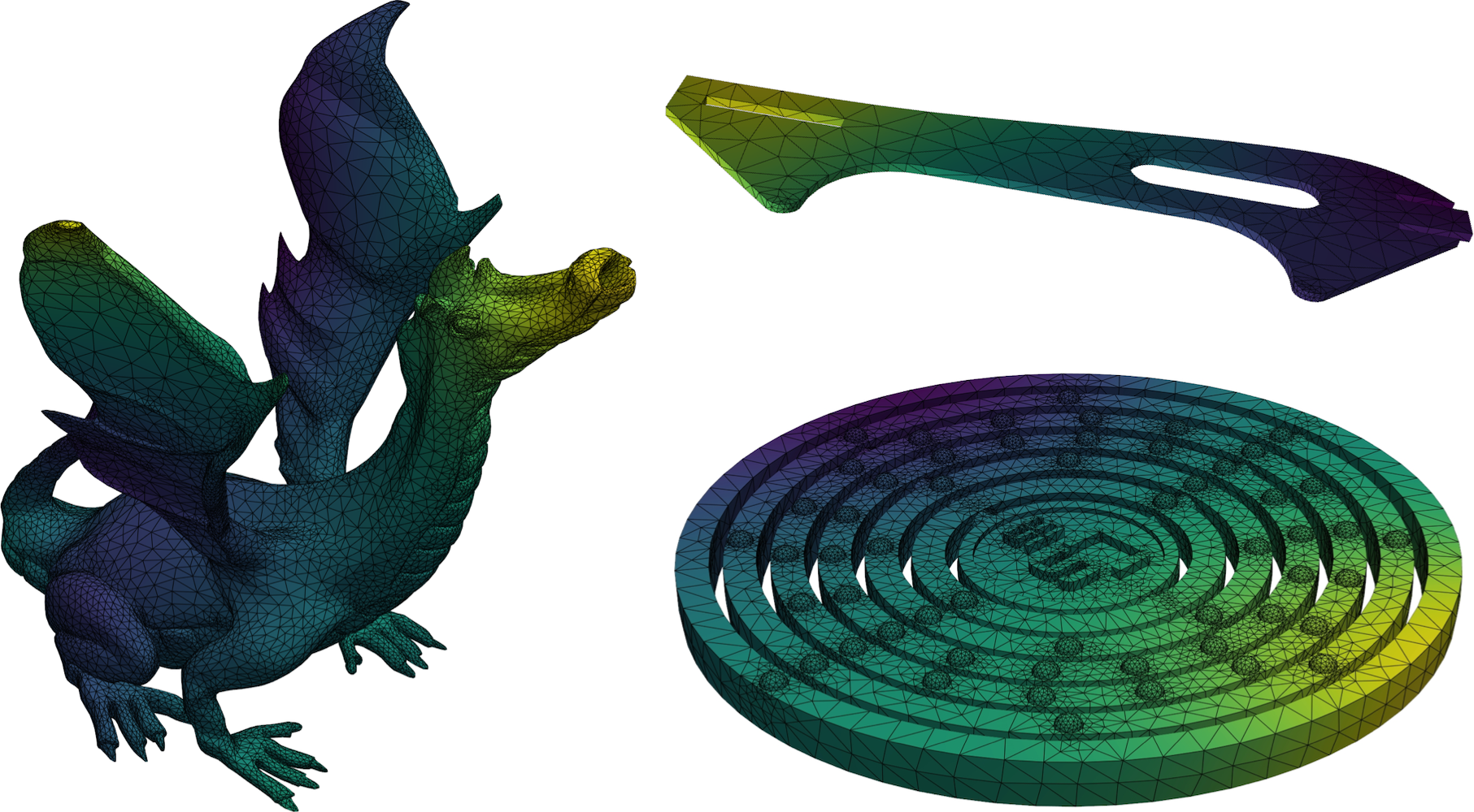
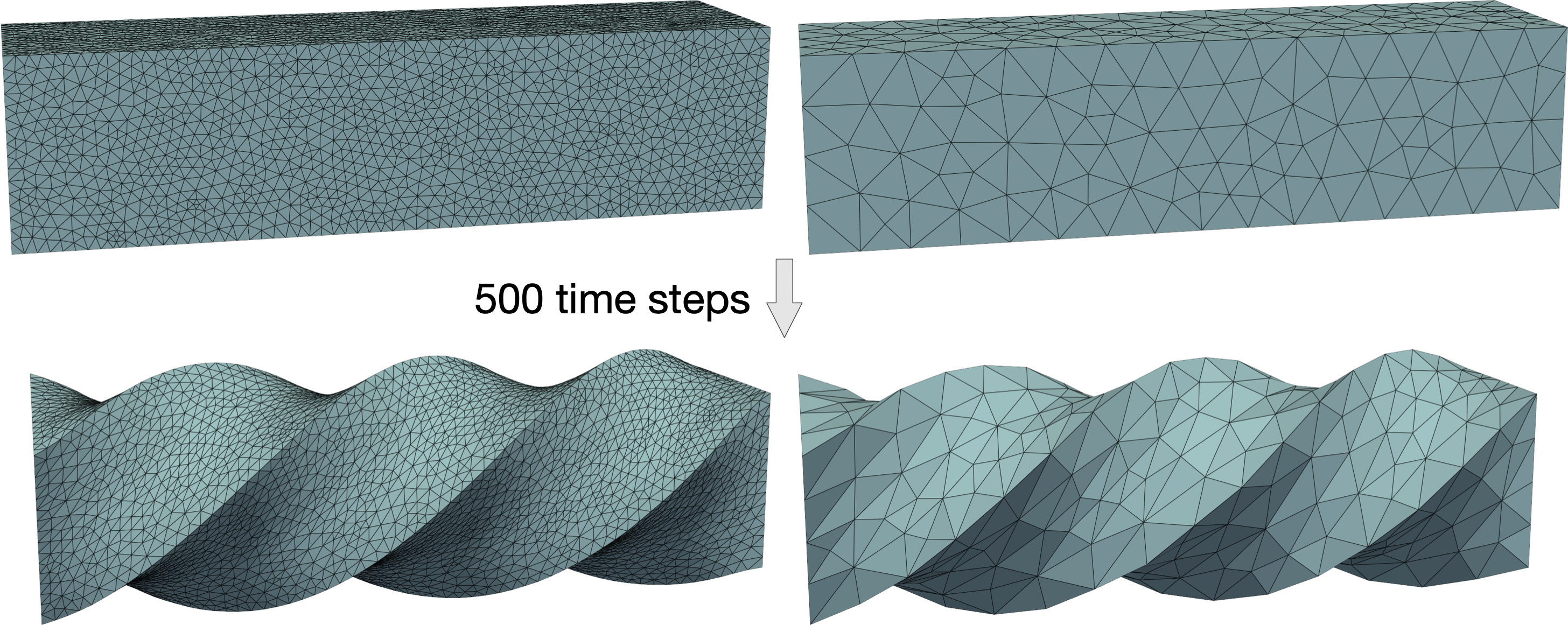
Across several test types—heat equation, Poisson equation, hyperelasticity (how materials deform), and synthetic matrices—their method:
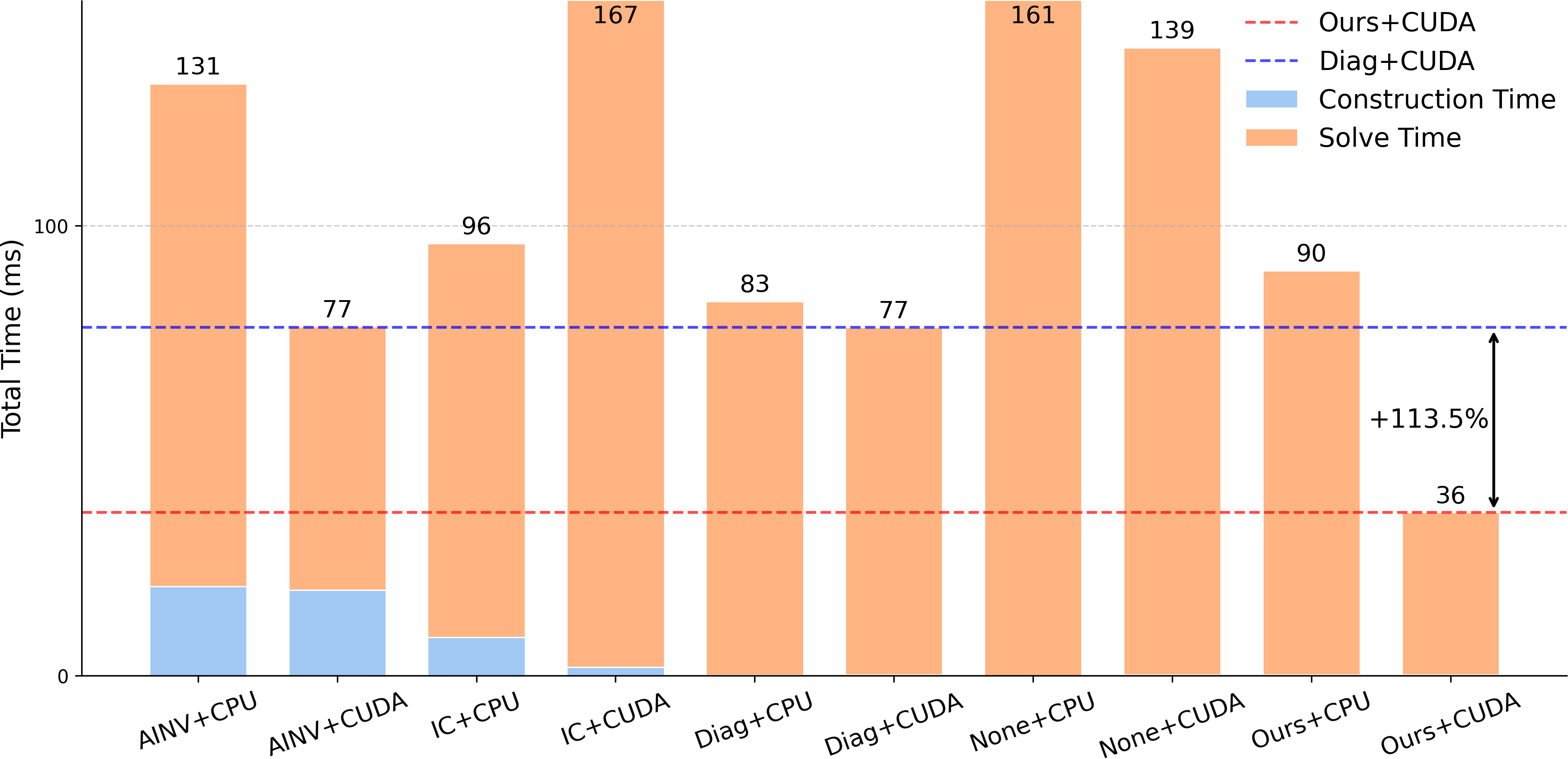
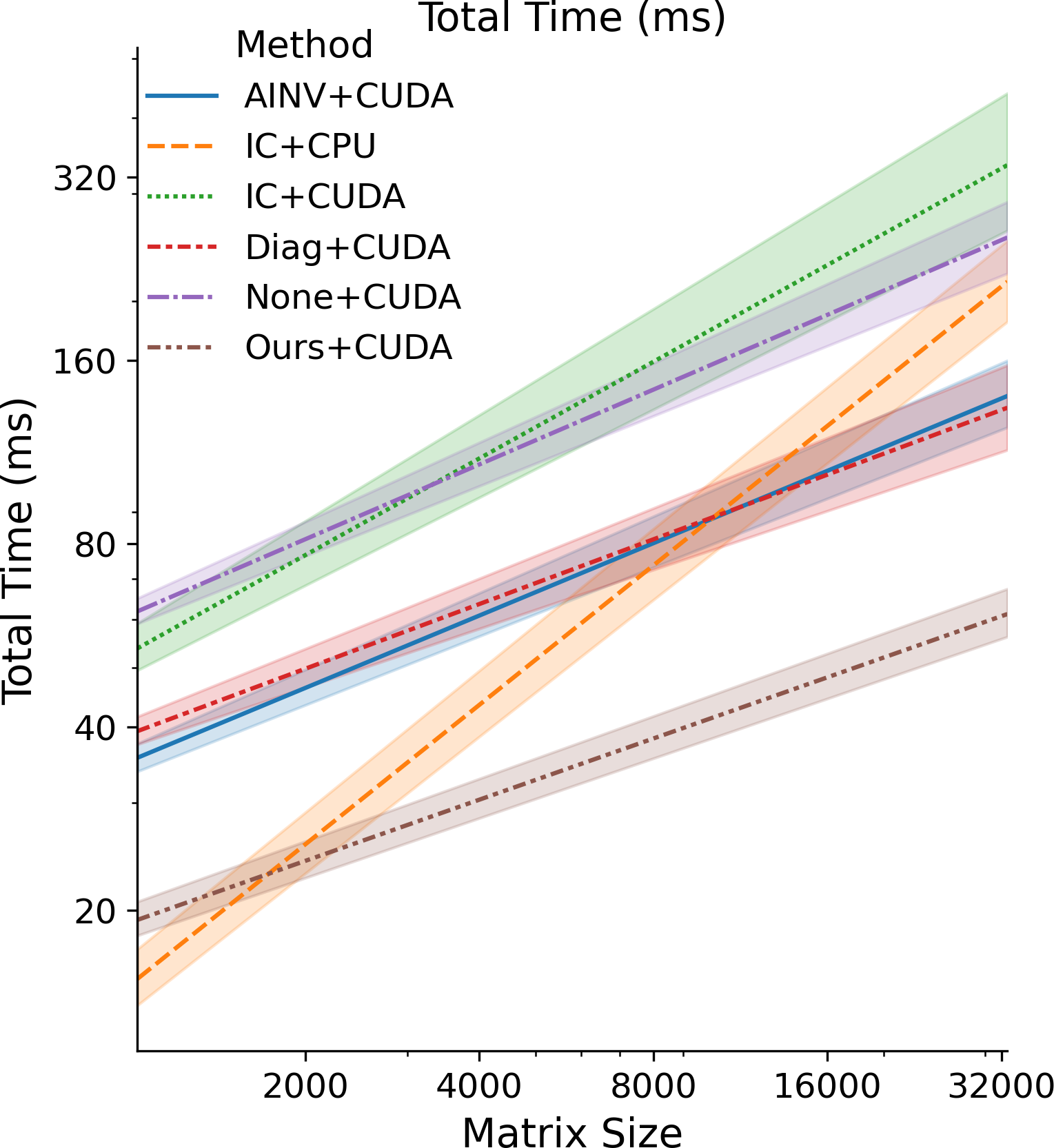
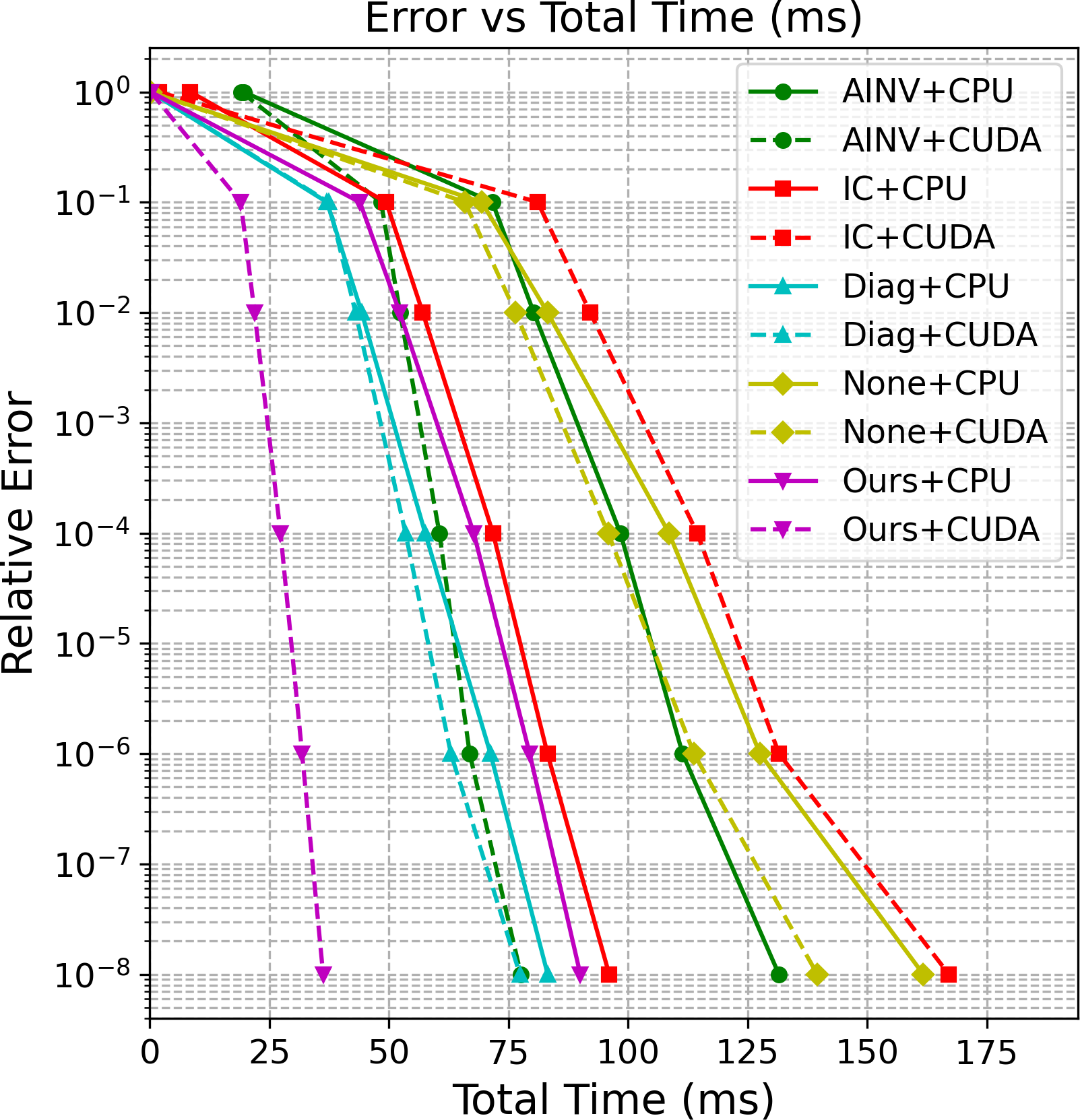
- Cut total GPU solve time by about 40–53% (roughly 1.7× to 2.1× speedup) compared to standard methods.
- Needed a similar or smaller number of CG steps than strong traditional preconditioners, but ran each step much faster on GPUs.
- Avoided triangular solves entirely; each CG step used only two sparse matrix–vector multiplications (a GPU sweet spot).
- Generalized well to new meshes, bigger problems, and different physical settings.
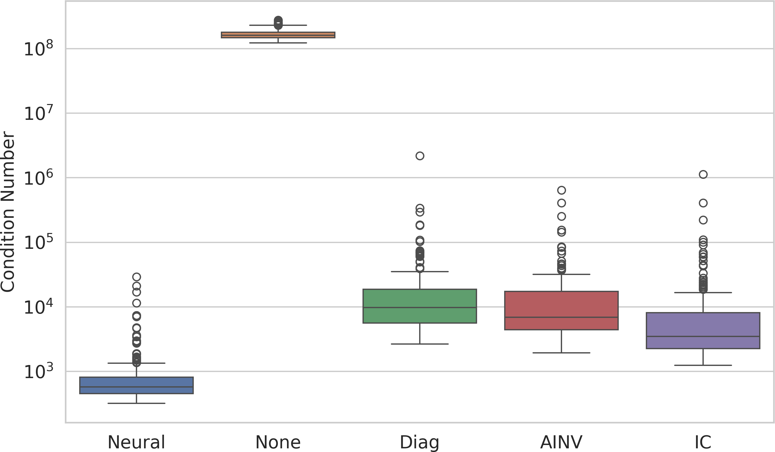
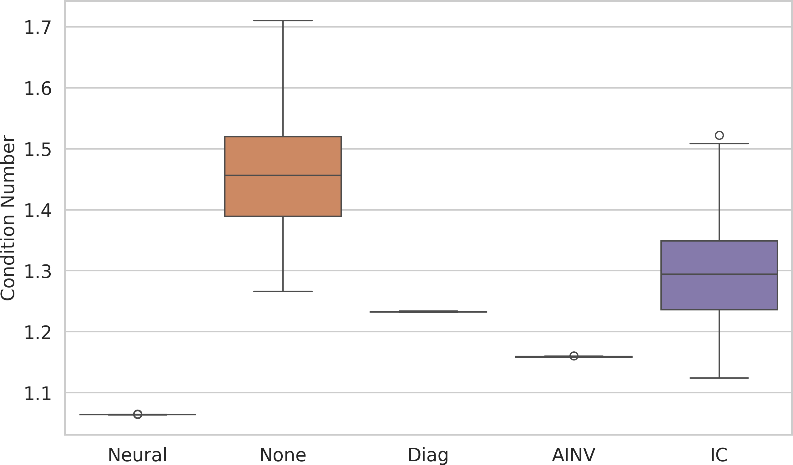
- Improved the condition number (a measure of how hard the system is), which is directly tied to CG’s speed.
Why this matters: Many scientific and engineering tasks depend on solving these large systems quickly. Faster solves on GPUs mean faster simulations, shorter training loops in physics-informed ML, and better use of modern hardware.
What could this change in the future?
This approach shows that:
- Learning GPU-friendly preconditioners can make large-scale simulations and scientific computing noticeably faster.
- Using GNNs for local, sparse structures (like SPAI) fits GPU hardware and the math of the problem well.
- Scale-aware training (SAI loss) can make models more robust and easier to train across many datasets.
Possible next steps include:
- Allowing the learned sparse pattern to expand beyond the original matrix for even better performance.
- Extending to other iterative solvers (like GMRES) and combining with multigrid methods.
- Scaling to multi-GPU systems for truly massive problems.
Overall, the paper delivers a practical, learnable, and GPU-ready way to speed up a core operation in scientific computing.
Knowledge Gaps
Knowledge gaps, limitations, and open questions
Below is a consolidated list of what remains missing, uncertain, or unexplored in the paper, phrased to guide concrete follow-up research:
- Lack of theoretical guarantees on spectral quality
- No bounds are provided on the condition number of the preconditioned system produced by the learned SPAI, nor on convergence rates of PCG under the proposed training objective.
- The paper enforces SPD via M⁻¹ = G Gᵀ + εI, but does not analyze how ε and the learned G jointly affect eigenvalue clustering or worst-case conditioning.
- Loss–theory mismatch and estimator design
- The SAI loss minimizes a Frobenius-norm proxy using Hutchinson probes, while the analysis bounding κ(AM⁻¹) invokes spectral norm; the connection between minimizing the empirical SAI loss and reducing κ in practice (and the size of the gap) is unquantified.
- The number and choice of probe vectors w, their variance, and estimator convergence vs. compute trade-offs are not specified or analyzed; guidance on probe budget for stable training is missing.
- The chosen normalization ‖A‖ = mean|A_ij| is ad hoc; comparisons to alternative scale-normalizations (e.g., spectral, Gershgorin/row-scaled, diagonal equilibration, per-block scaling) are not studied.
- Sparsity pattern selection remains fixed and heuristic
- G is constrained to share A’s sparsity pattern; there is no mechanism to learn or adapt sparsity (e.g., two-hop fill, adaptive pattern growth, memory-budgeted pattern selection, or differentiable top-k sparsification).
- No study of the trade-off between nnz(G), preconditioner quality, and GPU runtime; guidelines or automated strategies to allocate fill-ins under memory/latency constraints are missing.
- Limited scope: solver classes and matrix types
- The method is only evaluated on SPD systems with PCG; extensions to nonsymmetric or indefinite systems (e.g., GMRES, MINRES, BiCGSTAB) are untested.
- Behavior on near-singular SPD systems (e.g., pure Neumann problems), highly anisotropic coefficients, extreme ill-conditioning, or non-PDE SPD matrices is not assessed.
- Generalization breadth and domain shift
- Generalization beyond tetrahedral FEM/PDE-derived matrices (e.g., finite volume, discontinuous Galerkin, graph Laplacians with heavy-tailed degrees, kernel matrices) remains untested.
- Sensitivity to graph/matrix reorderings (RCM, METIS, nested dissection) and permutation robustness—both at train and test time—are not evaluated.
- Fairness and breadth of baselines
- Comparisons omit strong approximate inverse variants (e.g., FSAI with optimized patterns), polynomial preconditioners (Chebyshev/Jacobi–Chebyshev), and state-of-the-art GPU IC/triangular-solve implementations (e.g., supernodal, level-scheduled, batched solvers).
- AMG comparisons are relegated to the appendix; no systematic exploration of AMG configurations (coarsening, strength thresholds, smoothers) on GPU vs. the proposed method is provided.
- Ablation studies on model choices are minimal
- No ablation on GNN depth/width, number of message-passing layers, residual/normalization choices, or use of attention; the limits of “locality” (e.g., 2-hop vs. deeper) are not explored.
- Critical feature ablations (which node/edge features matter, geometry vs. purely algebraic inputs, block-wise vs. scalar features) are not reported.
- Hyperparameter sensitivity and tuning
- The impact of ε in M⁻¹ = G Gᵀ + εI on stability, conditioning, and runtime is not studied; no guidance on selecting ε across problems.
- The effect of block size b and block-structured decoding on quality vs. runtime is not analyzed.
- Dynamic and multi-RHS scenarios underexplored
- For time-evolving systems (e.g., hyperelasticity), strategies for incremental preconditioner updates (warm-starting G, low-rank corrections) are not investigated.
- Cost amortization and reuse across multiple right-hand sides (common in PDE workflows) are not quantified; the build-once/use-many setting could materially change trade-offs against factorization-based methods.
- Scale and systems limitations
- The approach is single-GPU only; there is no design or evaluation for multi-GPU/distributed settings (graph partitioning, communication overlaps, distributed GNN inference, distributed SpMV).
- Out-of-core training/inference strategies for very large matrices (10⁷–10⁸ DoF) are not addressed.
- Numerical precision and stability
- Robustness to mixed-precision arithmetic (FP16/TF32) on GPUs, error accumulation in two-SpMV preconditioner application, and training/inference quantization effects are not evaluated.
- Regularization of G (e.g., bounded weights, row/column scaling) to avoid pathological entries or loss of numerical stability is not discussed.
- Runtime decomposition details and kernel optimizations
- The impact of sparse format (CSR, ELL, HYB) selection, reordering for coalesced memory access, and kernel fusion for G and Gᵀ SpMVs is not explored; auto-tuning for SpMV performance is absent.
- Memory footprint comparisons (storing A and G vs. storing L, supernodes, or AMG hierarchies) and their implications on GPU occupancy are not provided.
- Measuring what matters: metrics and correlations
- The correlation between the SAI loss during training and the achieved κ(AM⁻¹) or PCG iteration counts across the full test suite is not systematically quantified.
- Condition numbers are demonstrated on a single small mesh; large-scale κ proxies (e.g., Lanczos-based spectral bounds) across datasets are missing.
- Data efficiency, training time, and robustness
- Training time, data efficiency (probes per matrix), variance across random seeds, and sensitivity to dataset size/diversity are not reported.
- Failure modes (e.g., when the learned preconditioner underperforms Diagonal) and safeguards (fallback selection or model uncertainty) are not discussed.
- Integration into broader solver stacks
- Use of the learned SPAI as a component in multigrid (e.g., as a smoother), in Newton–Krylov pipelines, or with domain decomposition (additive/multiplicative Schwarz) is only mentioned but not prototyped or evaluated.
- Reproducibility and deployment
- Detailed hyperparameters for Hutchinson probing, normalization choices per dataset, and training schedules are not fully specified; end-to-end training/inference wall-clock and memory profiles are not provided.
- Portability to common HPC libraries (PETSc, Trilinos) and integration overheads are not assessed.
Glossary
- Algebraic Multigrid (AMG): A multilevel preconditioning/solver technique that accelerates convergence by transferring error to coarser levels. "algebraic multigrid (AMG)"
- Approximate Inverse (AINV): A family of preconditioners that explicitly approximate the inverse of a matrix with a sparse structure. "Sparse Approximate Inverse (AINV)"
- Backward substitution: The process of solving an upper-triangular linear system by substituting from the last equation upward. "backward substitution "
- Blocked sparse matrix: A sparse matrix whose nonzero entries are organized as dense blocks, often used for systems with multiple variables per node. "for a blocked sparse matrix with as block size"
- Conjugate Gradient (CG): An iterative method for solving large, sparse, symmetric positive definite linear systems. "The conjugate gradient solver (CG) is a prevalent method"
- Condition number: A measure of how well-conditioned a matrix or system is; higher values generally mean slower or less stable convergence. "a lower condition number typically indicates faster CG convergence."
- Dirichlet boundary: A boundary condition specifying the value of the solution on the boundary of the domain. "Dirichlet boundary"
- Domain decomposition: A preconditioning/solver approach that partitions the computational domain into subdomains to improve scalability and performance. "domain decomposition \cite{smith1997domain} preconditioners"
- Elimination tree: A tree structure capturing dependency order during sparse matrix factorizations, influencing information flow and parallelism. "through the elimination tree"
- Finite Element Method (FEM): A numerical technique for solving PDEs by discretizing the domain into elements and forming a variational problem. "finite element method (FEM)"
- Forward substitution: The process of solving a lower-triangular linear system by substituting from the first equation downward. "forward substitution "
- GMRES: A Krylov subspace method for nonsymmetric linear systems that minimizes the residual over a growing subspace. "GMRES"
- Graph Neural Networks (GNNs): Neural models that operate on graph-structured data via local message passing and aggregation. "Graph Neural Networks (GNNs)"
- Hyperelasticity: A class of nonlinear solid mechanics models where stress derives from a strain energy function. "Hyperelasticity"
- Incomplete Cholesky (IC): A preconditioner formed by computing a sparse, incomplete Cholesky factorization, trading accuracy for efficiency. "Incomplete Cholesky (IC)"
- Krylov subspace methods: Iterative solvers that build approximations within the span of successive powers of the matrix applied to a vector. "other Krylov subspace methods such as GMRES"
- Mass matrix: A matrix representing mass distribution in discretized dynamics, typically appearing in second-order PDEs. "mass matrix"
- Message-passing layers: GNN layers in which nodes aggregate and transform information from their neighbors to update representations. "message-passing layers"
- Neo-Hookean material model: A common hyperelastic constitutive model for large deformation solid mechanics. "Neo-Hookean material model"
- Preconditioner: A matrix applied to transform a linear system into one that is easier for an iterative solver to converge on. "Preconditioners transform the original linear system into one easier to solve"
- Scale invariant Aligned Identity (SAI) loss: A loss that aligns the scaled preconditioned operator with the identity while being invariant to the magnitude of the input matrix. "Scale invariant Aligned Identity (SAI) loss"
- Scale invariance: A property where performance or behavior is unchanged under uniform scaling of inputs. "scale invariance property"
- Sparse Approximate Inverse (SPAI) preconditioner: A preconditioner that constructs a sparse matrix approximating the inverse, enabling efficient parallel application. "Sparse Approximate Inverse (SPAI) preconditioners"
- Sparse matrix-vector product (SpMV): The operation of multiplying a sparse matrix by a vector, a core kernel in iterative solvers. "The sparse matrix-vector product (SpMV) is the only routine required at each CG iteration"
- Spectral approximations: Approximations targeting the eigenvalue spectrum of an operator, crucial for preconditioning effectiveness. "spectral approximations"
- Stochastic trace estimator: A Monte Carlo method to estimate trace or Frobenius norms using random probe vectors. "stochastic trace estimator"
- Symmetric positive definite (SPD): A matrix class that is symmetric and has all positive eigenvalues, ensuring CG applicability. "symmetric positive definite(SPD) sparse linear systems"
- Triangular solves: Operations that solve lower/upper-triangular systems; often a parallelization bottleneck on GPUs. "two triangular solves at each CG step"
- Two-hop neighborhood: The set of nodes reachable in two edges from a given node, reflecting locality in graph computations. "two-hop neighborhood"
Practical Applications
Immediate Applications
The following applications can be deployed now with modest integration effort, leveraging the paper’s GPU-friendly learned SPAI preconditioners and the scale-invariant loss that trains using only the system matrix A.
- Sector: Engineering/CAE (FEM solvers for thermal, structural, elasticity)
- Use case: Drop-in GPU preconditioner for CG in commercial and in-house finite element solvers (e.g., thermal analysis, Poisson/heat, linear elasticity, hyperelasticity).
- Tools/products/workflows: Integrate a “Learned SPAI” module that takes the CSR of A and node/edge features, runs GNN inference to produce G, and applies M⁻¹ = GGᵀ + εI via two SpMV per CG iteration using cuSPARSE/cuBLAS. Train offline with SAI loss on representative meshes and PDE matrices; deploy with a fallback to IC/diagonal preconditioners.
- Impact: 40–53% reduction in GPU solve time (68–113% faster) observed across tested PDE-derived cases; better condition numbers and generalization to unseen meshes.
- Assumptions/dependencies: SPD sparse systems; GPU availability; representative training data for the solver’s domain; acceptable memory for G (same sparsity pattern as A in the current approach); ε tuning to enforce SPD.
- Sector: VFX/Interactive Graphics (real-time physics for animation/games)
- Use case: Faster CG for hyperelasticity and soft-body simulations in production pipelines and game engines.
- Tools/products/workflows: Pretrain on studio asset libraries (meshes/materials), run GNN inference per frame or per timestep to refresh preconditioners under remeshing; integrate into physics plugins for Unreal/Unity or in-house solvers.
- Impact: Lower latency for interactive rigs and simulation previews; paper shows a substantial speedup on hyperelasticity cases.
- Assumptions/dependencies: SPD system formation (common in normal-equation formulations); robust performance under changing meshes/topologies; GPU compute on artist workstations or render farms.
- Sector: Robotics (SLAM/pose graph optimization; mapping)
- Use case: Accelerate CG on normal equations in SLAM back-ends where matrices are SPD.
- Tools/products/workflows: ROS2 plugin that converts sparse normal matrices into graph features and builds G via GNN inference; applies SPAI in iterative solvers on embedded or desktop GPUs.
- Impact: Reduced optimization time per loop closure and faster map updates.
- Assumptions/dependencies: SPD normal-equation formulation; careful feature engineering for graph nodes/edges; manageable GPU memory on platforms like NVIDIA Jetson.
- Sector: Medical Imaging (CT/MRI iterative reconstruction)
- Use case: Speed up CG-based least-squares solves (SPD normal systems) in iterative reconstruction pipelines without changing reconstruction accuracy targets.
- Tools/products/workflows: Preconditioner builder that consumes A in CSR, trains using SAI loss, and deploys GPU SPAI for clinical pipelines; monitor convergence thresholds and total time T_total.
- Impact: Lower reconstruction times; improved throughput on GPU workstations.
- Assumptions/dependencies: SPD normal equations; adherence to clinical validation and QA; need domain-specific training data reflecting scan protocols.
- Sector: Machine Learning (Gaussian Processes, Kernel Ridge Regression)
- Use case: Faster CG for SPD kernel matrices in GPyTorch/Scikit-learn pipelines with large datasets.
- Tools/products/workflows: GPyTorch extension providing learned SPAI preconditioner for K; training requires only A (kernel matrix), not labels; runtime uses two SpMV per iteration.
- Impact: Fewer iterations and lower end-to-end inference/training times in large-kernel regimes.
- Assumptions/dependencies: SPD kernels (e.g., RBF/Matern); memory constraints for large K; stable scaling with SAI loss.
- Sector: Network Science/Data Analytics (Graph Laplacian solves)
- Use case: Accelerate Laplacian linear system solves (e.g., semi-supervised learning, spectral clustering).
- Tools/products/workflows: Plugin for graph analytics libraries (GraphBLAS/NetworKit) that generates a learned SPAI from Laplacian A and applies preconditioning on GPUs.
- Impact: Faster graph signal processing and ranking tasks at scale.
- Assumptions/dependencies: SPD Laplacians; graph features available for GNN; sufficient GPU memory bandwidth.
- Sector: Cloud/HPC Services
- Use case: “Preconditioner-as-a-Service” that returns G for uploaded sparse SPD matrices, enabling users to accelerate CG without building ML infrastructure.
- Tools/products/workflows: Service API that ingests CSR A and metadata, trains once per domain (using SAI loss), caches models, and serves G generation; integrates with cuSPARSE/cuBLAS on the client side.
- Impact: Immediate acceleration for SaaS PDE solvers and digital-twin workloads; reduced energy costs via shorter runs.
- Assumptions/dependencies: Data security/privacy for matrices; representative domain models; quantification of energy savings vs. training cost.
- Sector: Academia/Education
- Use case: Teaching and research tool for GPU-friendly preconditioning in numerical linear algebra courses and labs.
- Tools/products/workflows: Open-source example notebooks and CUDA/C++ bindings; experiments comparing diagonal, IC, traditional SPAI, and learned SPAI; reproducible benchmarks.
- Impact: Hands-on understanding of preconditioning trade-offs and GNN-based approaches; accessible ~24k-parameter models simplify instruction.
- Assumptions/dependencies: Availability of GPUs in labs; datasets of SPD matrices; basic ML tooling.
Long-Term Applications
The following applications require additional research, scaling, or development beyond the paper’s current scope.
- Sector: HPC/Scientific Computing — Multi-GPU and Distributed SPAI-GNN
- Use case: Preconditioning extremely large SPD systems (city-scale digital twins, climate models) via distributed GNN training/inference and multi-GPU application of M⁻¹.
- Tools/products/workflows: Partitioned sparse graph inputs, distributed message passing with NCCL/NVLink, overlap of communication and SpMV; integration into MPI-based solvers.
- Dependencies/assumptions: Robust partitioning strategies, communication-efficient graph learning, memory-aware sparsity management; research needed for scalability and resilience.
- Sector: General Solvers — Beyond SPD (GMRES and nonsymmetric/indefinite)
- Use case: Extend learned SPAI to GMRES and nonsymmetric systems common in CFD and transport problems.
- Tools/products/workflows: New architectures and loss functions for nonsymmetric matrices; validation in industrial codes (e.g., combustion, power systems).
- Dependencies/assumptions: Stability guarantees without SPD constraints; careful spectral control; potential hybridization with other preconditioners.
- Sector: Solver Quality — Adaptive/learned sparsity patterns
- Use case: Learn or auto-tune sparsity beyond “same pattern as A” (e.g., two-hop stencils, drop tolerances) to balance preconditioner quality and memory footprint.
- Tools/products/workflows: Pattern-search optimizer or RL-based sparsity controller; runtime adaptation driven by matrix statistics.
- Dependencies/assumptions: Memory budgets; guardrails to prevent overfitting and instability; compatibility with SpMV kernels.
- Sector: Multigrid — ML-AMG hybrids
- Use case: Use learned SPAI as smoother or coarse-grid operator in AMG to improve robustness and reduce parameter tuning.
- Tools/products/workflows: Integration with PyAMG/AmgX, automated learning of coarsening and smoothing policies; RL for threshold tuning.
- Dependencies/assumptions: Theoretical guarantees for convergence and stability; domain-specific validation.
- Sector: Differentiable Simulation and Inverse Design
- Use case: Make SPAI preconditioning differentiable for end-to-end training of PDE-constrained optimization, inverse problems, and neural operators.
- Tools/products/workflows: Differentiable SpMV and loss formulations; integration with JAX/PyTorch for gradient flow through solvers.
- Dependencies/assumptions: Stable gradients; trade-offs between solver speed and differentiability overhead.
- Sector: Hardware/Systems — Mixed-precision and auto-tuning
- Use case: Combine learned SPAI with mixed-precision CG and RL-driven precision tuning to minimize time and energy in production.
- Tools/products/workflows: Precision controllers, confidence-driven precision selection; co-design with GPU kernels for SpMV.
- Dependencies/assumptions: Numerical stability under precision changes; hardware-specific optimization; rigorous QA for safety-critical domains.
- Sector: Policy/Standards — Benchmarking, energy, and procurement
- Use case: Establish preconditioning benchmarks and energy KPIs for GPU solvers in public HPC centers and regulated industries (e.g., medical).
- Tools/products/workflows: Standard test suites for SPD systems; reporting protocols for T_total, energy savings, and robustness; certification pathways.
- Dependencies/assumptions: Community adoption; reproducible metrics; alignment with regulatory bodies for safety and reliability.
- Sector: Edge/Embedded — Robotics and autonomous systems
- Use case: Deploy compact learned SPAI preconditioners on embedded GPUs for low-latency control and planning (e.g., SLAM, real-time mapping).
- Tools/products/workflows: Memory-efficient versions of G and model compression; on-device incremental training or adaptation.
- Dependencies/assumptions: Tight memory/power budgets; real-time constraints; robust adaptation to nonstationary environments.
- Sector: Open-source Ecosystem — Integration into core libraries
- Use case: Incorporate learned SPAI preconditioners into cuSPARSE/PyAMG and other solver stacks to broaden impact.
- Tools/products/workflows: Stable APIs that accept CSR matrices and return CSR G; sample models for common PDE classes; continuous benchmarking CI.
- Dependencies/assumptions: Maintainer buy-in; long-term support; documented failure modes and fallback strategies.
Collections
Sign up for free to add this paper to one or more collections.

