Convex optimization (2106.01946v4)

Abstract: This textbook is based on lectures given by the authors at MIPT (Moscow), HSE (Moscow), FEFU (Vladivostok), V.I. Vernadsky KFU (Simferopol), ASU (Republic of Adygea), and the University of Grenoble-Alpes (Grenoble, France). First of all, the authors focused on the program of a two-semester course of lectures on convex optimization, which is given to students of MIPT. The first chapter of this book contains the materials of the first semester ("Fundamentals of convex analysis and optimization"), the second and third chapters contain the materials of the second semester ("Numerical methods of convex optimization"). The textbook has a number of features. First, in contrast to the classic manuals, this book does not provide proofs of all the theorems mentioned. This allowed, on one side, to describe more themes, but on the other side, made the presentation less self-sufficient. The second important point is that part of the material is advanced and is published in the Russian educational literature, apparently for the first time. Third, the accents that are given do not always coincide with the generally accepted accents in the textbooks that are now popular. First of all, we talk about a sufficiently advanced presentation of conic optimization, including robust optimization, as a vivid demonstration of the capabilities of modern convex analysis.

• The paper introduces convex optimization’s theoretical framework, efficient algorithms, and robust numerical methods for solving optimization problems.
• It explains key concepts such as convex sets, duality theory, and conditions for optimality that underpin modern optimization techniques.
• The paper highlights practical applications in optimal transport, control systems, and machine learning, demonstrating actionable insights.

Convex Optimization: Theory, Algorithms, and Applications

Convex optimization constitutes a fundamental discipline within applied mathematics, providing a robust framework for formulating and solving a wide array of optimization problems. Its significance stems from the rich theoretical properties of convex functions and sets, which enable the development of provably efficient algorithms, a feature often absent in general non-convex optimization. Historically, the roots of convexity trace back to ancient Greek geometry, with rigorous mathematical development gaining traction in the 19th and 20th centuries through the works of Cauchy, Minkowski, Fenchel, and Rockafellar. The practical imperative for convex optimization emerged prominently in the mid-20th century, driven by economic and military planning problems that led to the genesis of linear programming. The field is fundamentally supported by three pillars: foundational theory (e.g., convex analysis), sophisticated mathematical modeling, and computationally efficient numerical methods.

Core Concepts of Convex Analysis

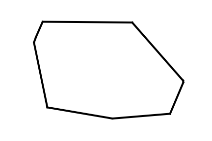
The bedrock of convex optimization is defined by convex sets and convex functions. A set $Q$ is convex if, for any two points $x, y \in Q$, the entire line segment connecting them also lies within $Q$. Formally, $$\forall x, y \in Q, \forall \alpha \in [0, 1] \implies \alpha x + (1-\alpha) y \in Q$$. This property extends to any convex combination of points within the set. Geometrically, this implies that a convex set has no "indentations" or "holes" (Figure 1).

Figure 1: An example of a convex set.

A function $f: \mathbb{R}^n \to \mathbb{R}$ is convex if its domain is a convex set and for any $x, y$ in its domain, Jensen's inequality holds: $$f(\alpha x + (1-\alpha) y) \leq \alpha f(x) + (1-\alpha) f(y)$$ for all $\alpha \in [0, 1]$. Equivalently, a function is convex if and only if its epigraph, epi $$f = \{ (x, \alpha) \in \text{dom } f \times \mathbb{R} \mid \alpha \ge f(x) \}$$, is a convex set. For twice-differentiable functions, convexity is characterized by the positive semi-definiteness of its Hessian matrix, $\nabla^2 f(x) \succeq 0$.

Cones and Generalized Inequalities

Cones are special types of sets. A set $K$ is a cone if for any $x \in K$ and $\lambda \ge 0$, $\lambda x \in K$. A convex cone is simply a cone that is also a convex set. Proper (or regular) cones are convex cones that are also closed, have a non-empty interior, and are pointed (i.e., contain no lines). Proper cones induce generalized inequalities, $x \succeq_K y \iff x - y \in K$, which define partial order relations in vector spaces. Key examples of proper cones include the non-negative orthant $\mathbb{R}_+^n$, the Lorentz cone (also known as the ice-cream cone) $L^n$, and the cone of positive semidefinite matrices $\mathbb{S}_+^n$. The dual cone $K^*$ of a cone $K$ is defined as $$K^* = \{ p \in V^* \mid \langle x,p \rangle \geq 0 \ \forall x \in K \}$$. For proper cones, $K^*$ is also a proper cone, and $(K^*)^* = K$.

Operations Preserving Convexity

Several fundamental operations preserve the convexity of sets and functions, which is crucial for building complex convex optimization problems from simpler components. These include:

• Non-negative weighted sums: A non-negative weighted sum of convex functions is convex.
• Affine transformations: If $f(x)$ is convex, then $g(x) = f(Ax+b)$ is also convex.
• Pointwise maximum/supremum: The pointwise maximum of any collection (finite or infinite) of convex functions is convex. This is a powerful property for formulating many practical problems, including those involving worst-case scenarios.
• Minimization: If $G(x,y)$ is convex in $(x,y)$ and $Q$ is a convex set, then $f(x) = \inf_{y \in Q} G(x,y)$ is convex in $x$.

Nonsmooth Optimization and Subgradients

While smoothness (differentiability) simplifies optimization, many practical convex problems involve non-differentiable functions. For convex functions, the concept of a subgradient generalizes the gradient for non-differentiable points. The subdifferential $\partial f(x_0)$ of a convex function $f$ at $x_0$ is the set of all subgradients $g$ such that $f(x) - f(x_0) \ge g^T (x - x_0)$ for all $x$ in the domain. For a convex function, a point $x^*$ is a global minimum if and only if $0 \in \partial f(x^*)$ (Fermat's Theorem for convex functions). Operations on subdifferentials, such as for sums of functions or affine transformations, simplify the analysis of non-smooth problems. Danskin's Theorem provides conditions for the differentiability (or subgradient calculation) of a function defined as the maximum (or minimum) over another variable.

Duality Theory and Optimality Conditions

Duality theory provides a powerful lens through which to analyze and solve optimization problems. For a general optimization problem with equality and inequality constraints, the Lagrangian function is defined as $$L(x, \lambda, \nu) = f(x) + \sum_{i} \lambda_i g_i (x) + \sum_{j} \nu_j h_j (x)$$, where $\lambda_i$ and $\nu_j$ are Lagrange multipliers associated with equality and inequality constraints, respectively. The dual function is given by $$\varphi(\lambda, \nu) = \inf_{x} L(x, \lambda, \nu)$$. A fundamental property is weak duality: $\varphi(\lambda, \nu) \le f^*$ for any feasible $\nu \ge 0$, where $f^*$ is the optimal primal objective value. The duality gap is defined as $f^* - \varphi^*$, where $\varphi^*$ is the optimal dual objective value.

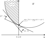
Figure 2: Geometric interpretation of the existence of Lagrange multipliers for a convex programming problem.

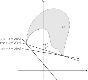
Strong duality, where $f^* = \varphi^*$, holds under certain conditions, such as Slater's condition for convex programs. This implies that there is no "duality gap" (Figure 3).

Figure 3: Three supporting hyperplanes corresponding to three values of the dual function. Case of a problem with one inequality constraint: $\min\limits_{h(x) \, \le \, 0} f(x)$.

The Karush-Kuhn-Tucker (KKT) conditions are necessary optimality conditions for differentiable convex problems, and under Slater's condition, they are also sufficient. These conditions include stationarity of the Lagrangian with respect to the primal variables, primal and dual feasibility, and complementary slackness ($\nu_j^* h_j(x^*) = 0$ for inequality constraints). Sensitivity analysis, often utilizing Lagrange multipliers, provides insights into how the optimal objective value changes with small perturbations in the problem constraints.

Specialized Convex Programs

Several important classes of convex optimization problems arise from specific forms of objective functions and constraints:

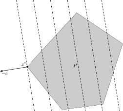
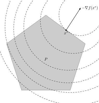
• Linear Programming (LP): Minimizing a linear objective function subject to linear equality and inequality constraints. LP problems are widely used in resource allocation, logistics, and planning. Pioneers include Leonid Kantorovich and George Dantzig. The simplex method is a classic algorithm, though it can exhibit exponential worst-case performance (e.g., Klee-Minty cube examples). Interior-point methods offer polynomial-time guarantees for LP.

  Figure 4: Geometric interpretation of a linear programming problem. P - feasible set (polyhedron), objective function $c^T x$ is linear (its level lines are shown by dotted lines - these are hyperplanes orthogonal to vector $c$, the value of the objective function decreases in the direction of the antigradient -c, therefore the optimal point $x^*$ is the point of the polyhedron P in the direction -c, where the level line becomes tangent to P).

• Quadratic Programming (QP): Minimizing a convex quadratic objective function subject to linear constraints. This is a common class found in various applications, including support vector machines and control.

  Figure 5: Example of a graphical representation of a quadratic optimization problem. Feasible set $P = \{x \, | \, Ax \le b \}$, level lines of the objective function $f$ are shown by dotted lines. The solution to the problem is point $x^*$.

• Conic Programming (CP): A highly general class where the linear inequalities are replaced by generalized inequalities defined by convex cones.
  • Second-Order Cone Programming (SOCP): Involves generalized inequalities defined by Lorentz cones.
  • Semidefinite Programming (SDP): Involves generalized inequalities defined by the cone of positive semidefinite matrices.

Conic programming provides a unified framework for many convex problems and can often lead to efficient solution methods via interior-point algorithms. Many non-convex problems, especially from combinatorial optimization, can be effectively approximated using SOCP or SDP relaxations, often with performance guarantees. For instance, the MaxCut problem can be relaxed into an SDP, providing a strong approximation bound.

Robust Optimization

In real-world applications, parameters defining an optimization problem are rarely known with perfect certainty. Robust optimization (RO) provides a methodology to explicitly account for such uncertainty in the problem data. Instead of solving a single deterministic problem, RO seeks solutions that are feasible and optimal for all possible realizations of uncertain parameters within a predefined "uncertainty set". For convex uncertainty sets, robust counterparts of many convex problems can often be formulated as larger, but still tractable, convex programs, particularly as conic programs. This approach ensures solution robustness against data variations, preventing feasibility violations that might arise from small perturbations.

Efficiency of Numerical Optimization Methods

The efficiency of numerical optimization algorithms is often analyzed within the "black-box" or "oracle" model. This model assumes that the algorithm interacts with the objective function and constraints only through an oracle that provides function values, gradients, or higher-order derivatives at queried points. The computational complexity is then measured by the number of oracle calls required to achieve a desired solution accuracy.

For smooth convex optimization problems, Nesterov's accelerated gradient methods achieve optimal convergence rates. For non-smooth convex problems, subgradient methods are optimal. Interior-point methods, particularly tailored for conic programming, also offer polynomial-time complexity guarantees.

Methods for Small-Scale Convex Optimization

For problems with relatively low dimensionality ($n$), methods like the ellipsoid method offer polynomial-time convergence guarantees. The ellipsoid method iteratively refines a region known to contain the optimum by repeatedly cutting an ellipsoid containing the current search space. Its theoretical complexity is $O(n^2 \log(1/\varepsilon))$ oracle calls for $\varepsilon$-accuracy, making it a theoretically significant, though often practically slower, alternative to other methods for very high precision.

First-Order Methods for Smooth Convex Optimization

Gradient descent is a foundational first-order method. For smooth convex functions with Lipschitz-continuous gradients, it converges at a rate of $O(1/N)$ in terms of function value error after $N$ iterations. For strongly convex functions, it achieves linear convergence. However, Nesterov's accelerated gradient methods dramatically improve these rates, achieving $O(1/N^2)$ for smooth convex functions and linear convergence with a condition number dependency of $O(\sqrt{L/\mu} \log(1/\varepsilon))$ for strongly convex functions. These methods often involve auxiliary sequences and specific step-size rules to achieve optimal acceleration. Recent developments include tensor methods (higher-order derivatives) and meta-algorithms that unify and accelerate various first-order schemes.

Applications of Convex Optimization

Convex optimization finds widespread application across diverse scientific and engineering domains:

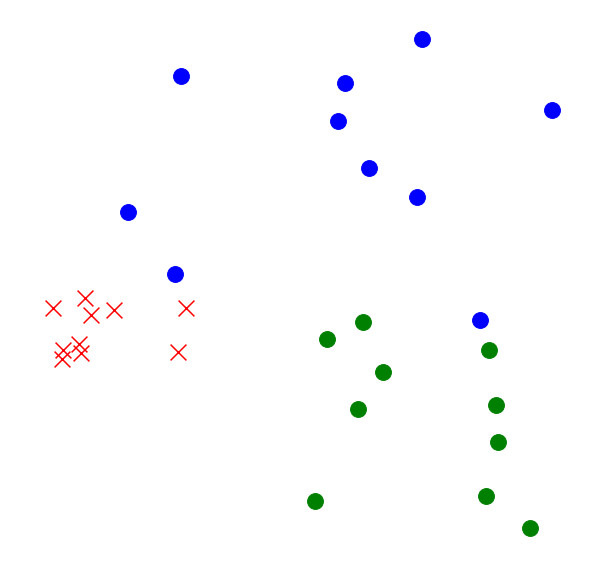
• Optimal Transport (OT): The Monge-Kantorovich problem, defining the Wasserstein distance between probability measures, quantifies the minimal cost to transform one distribution into another. This has found applications in image processing, machine learning (e.g., Generative Adversarial Networks), and comparing complex datasets (Figure 6, 20). Computing Wasserstein distance and barycenters (average distributions) is an active research area, often involving entropic regularization and specialized optimization algorithms.

  Figure 6: Which clusters of points are closer to each other - blue circles to green circles or blue circles to red crosses?

  

Figure 7: How to calculate the distance from Russia to France?

• System Identification and Control: Optimal experiment design involves selecting input signals to maximize the precision of system parameter estimation. This often translates into semidefinite programming problems where Fisher information matrices are maximized subject to signal energy constraints.
• Structural Optimization (e.g., Truss Topology): Designing lightweight and rigid structures involves minimizing material usage subject to load-bearing constraints. This can be formulated as a semidefinite program, where masses of potential structural elements are optimized.
• Anomaly Detection: Identifying unusual data points by fitting a minimal volume ellipsoid or other simple convex shapes around "normal" data.
• Signal Processing: Many signal processing problems, such as sparse approximation or denoising, can be cast as convex optimization problems, often utilizing $\ell_1$-norm regularization (LASSO).
• Polynomial Optimization: While generally non-convex, problems involving polynomials can be approximated using hierarchies of semidefinite programs based on sums of squares (SOS) polynomials or moment relaxations. These provide increasingly tight lower bounds on the global optimum.

Computational Aspects and Software

The practical applicability of convex optimization relies heavily on efficient numerical solvers and modeling tools.

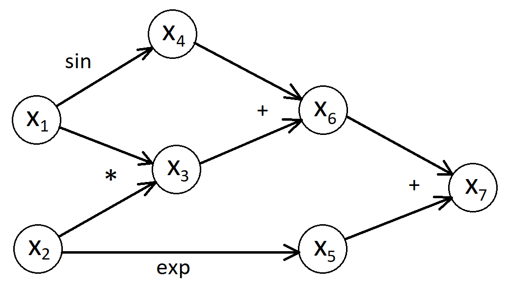
• Automatic Differentiation (AD): AD techniques enable the precise computation of gradients and higher-order derivatives of complex functions defined by computer programs. This is fundamental for gradient-based optimization algorithms and forms the backbone of modern machine learning frameworks like TensorFlow and PyTorch. AD propagates derivatives through a computational graph (Figure 8) in either forward or reverse mode. The reverse mode (backpropagation) is particularly efficient for functions with many inputs and a scalar output.

  Figure 8: Computational graph of the function $f(x_1, \, x_2) = x_1 x_2 + \sin x_1 + e^{x_2}$.

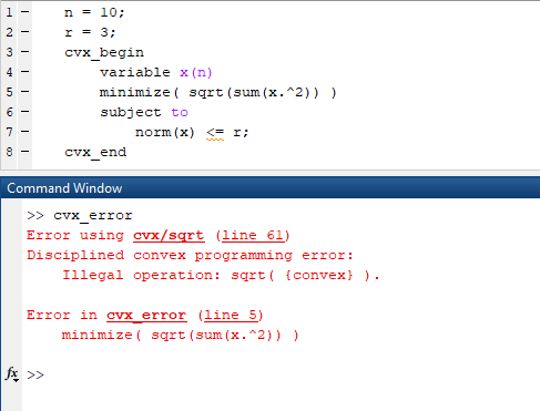
• Optimization Software: High-quality solvers for various convex programming classes are widely available. Packages like CVX (for MATLAB), CVXPY (for Python), and Convex.jl (for Julia) provide user-friendly interfaces for "disciplined convex programming" (DCP), automatically converting problems into standard conic forms solvable by specialized solvers (e.g., SDPT3, SeDuMi, MOSEK, Gurobi). This abstraction allows users to focus on problem modeling rather than algorithmic details. However, an improperly formulated problem, even if convex, might be rejected by the DCP framework (Figure 9).

  Figure 9: Example of an incorrect problem formulation for the CVX package.

Conclusion

Convex optimization continues to be a cornerstone of mathematical programming, with ongoing theoretical advancements and expanding real-world applications, particularly in the era of large-scale data analysis and machine learning. Its enduring relevance is tied to the inherent tractability of convex problems and the continuous innovation in numerical algorithms, many of which are described as increasingly universal and adaptive. The robust theoretical underpinnings, combined with powerful computational tools, ensure its continued central role in addressing complex challenges across various domains.