Terminal Velocity Matching
Abstract: We propose Terminal Velocity Matching (TVM), a generalization of flow matching that enables high-fidelity one- and few-step generative modeling. TVM models the transition between any two diffusion timesteps and regularizes its behavior at its terminal time rather than at the initial time. We prove that TVM provides an upper bound on the $2$-Wasserstein distance between data and model distributions when the model is Lipschitz continuous. However, since Diffusion Transformers lack this property, we introduce minimal architectural changes that achieve stable, single-stage training. To make TVM efficient in practice, we develop a fused attention kernel that supports backward passes on Jacobian-Vector Products, which scale well with transformer architectures. On ImageNet-256x256, TVM achieves 3.29 FID with a single function evaluation (NFE) and 1.99 FID with 4 NFEs. It similarly achieves 4.32 1-NFE FID and 2.94 4-NFE FID on ImageNet-512x512, representing state-of-the-art performance for one/few-step models from scratch.

Paper Prompts
Sign up for free to create and run prompts on this paper using GPT-5.
Top Community Prompts
Explain it Like I'm 14
Explaining “Terminal Velocity Matching” for a 14-year-old
Overview
This paper introduces a new way to train image-generating AI models so they can make high-quality pictures very quickly—often in just one step. The method is called Terminal Velocity Matching (TVM). It helps models learn to go directly from “noise” (random pixels) to clear images without needing dozens of tiny steps, which makes generation faster and more efficient.
What questions does the paper try to answer?
The paper focuses on a few simple but important questions:
- Can we train a model in one stage so it makes great images in just one or a few steps?
- Can we connect this fast method to solid math guarantees about how close the generated images are to real ones?
- Can we keep training stable and efficient for big models like transformers?
- Can we make it work at high resolutions (big images) without slowing down too much?
How does the method work?
Think of generating an image like traveling from a starting point (random noise) to a destination (a real-looking image). Many popular methods take lots of small steps to get there. TVM aims to “jump” further, doing the trip in one or only a few steps.
Here’s the core idea using everyday language:
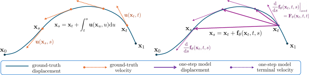
- Flow Matching (older method) learns the “instant speed” at the start of the trip. Imagine you measure how fast you start moving.
- TVM learns the “speed at the end” of the jump, called terminal velocity. That’s like ensuring you arrive moving in the right direction and speed at the destination point. If the speed at the end matches the true path, the whole jump is likely correct.
How they make this practical:
- They use a model that takes two times: a start time and an end time. This lets the model learn to jump between any moments, not just slowly step forward.
- They combine two learning goals: 1) Learn the normal “instant speed” at any single time (like Flow Matching). 2) Make sure the “end speed” after a jump matches what the true path would have (Terminal Velocity Matching).
- They provide a mathematical guarantee: if the model’s layers behave smoothly (no wild jumps when inputs change a little), the TVM training objective gives an upper bound on a distance called the “2-Wasserstein distance.” You can think of this distance as a way to measure how close the model’s image distribution is to the real image distribution. Smaller is better.
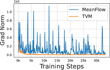
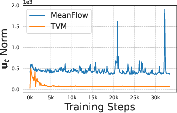
Making it stable and fast:
- Transformers (a type of AI model) sometimes aren’t “smooth” enough, which can cause training to blow up. The authors make small changes (like using RMSNorm and normalizing certain parts) to keep the model smooth and stable.
- They create a faster attention kernel (a piece of code for the model’s attention mechanism) that efficiently computes how the model’s output changes with time. This speeds up training and reduces memory use.
- They handle “classifier-free guidance” (CFG), a common trick that improves image quality by steering the model toward a class label. They design the training and the network outputs so different guidance strengths are stable and don’t cause huge gradients.
Sampling (how you actually make images):
- With TVM, you can choose one step (super fast) or a few steps (still fast but slightly better). You just run the model with selected start and end times and add the predicted jump.
What did they find?
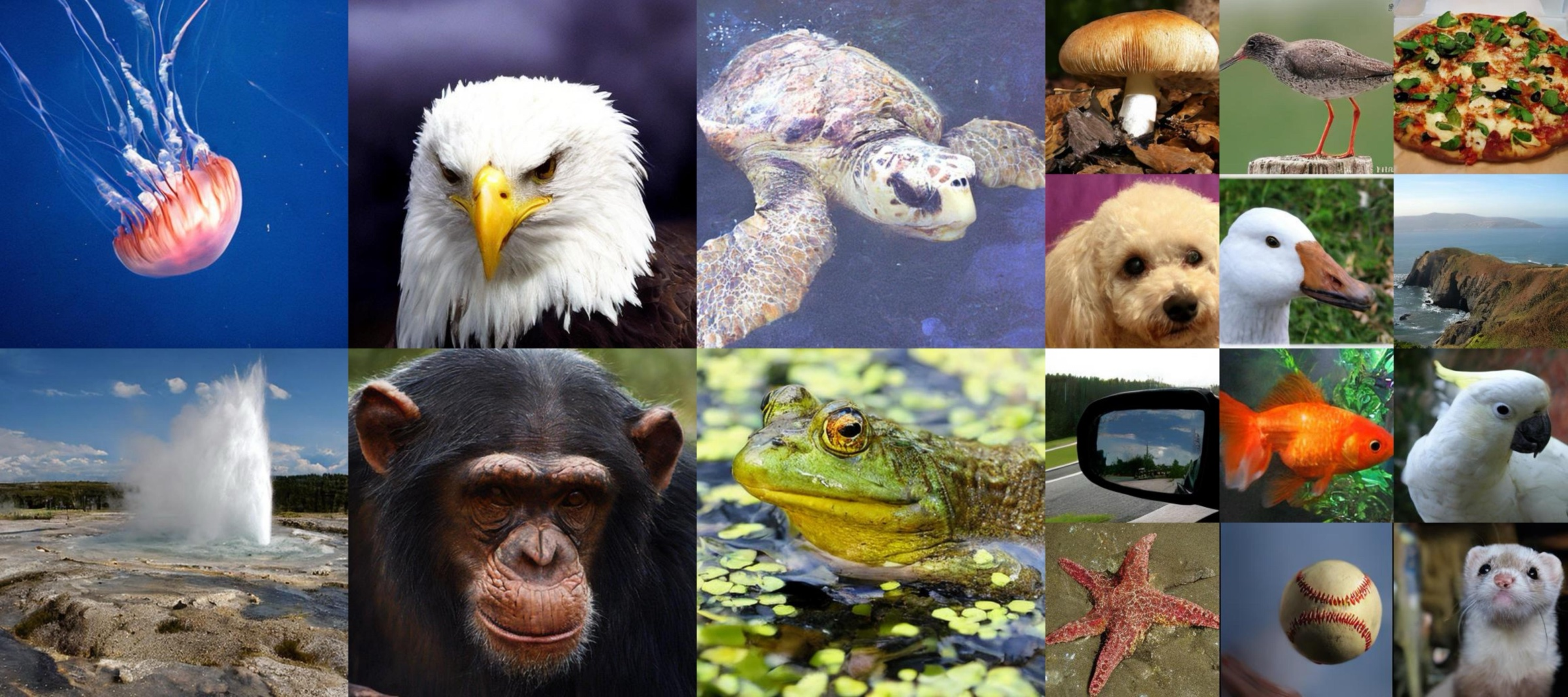
The authors tested TVM on ImageNet, a well-known dataset for image generation, at two resolutions: 256×256 and 512×512. They report FID scores (a popular metric where lower is better; it measures how “real” generated images look).
Main results:
- At 256×256:
- 1 step: TVM gets an FID of 3.29, beating other from-scratch methods.
- 4 steps: TVM gets an FID of 1.99, matching or beating strong diffusion baselines that use hundreds of steps.
- At 512×512:
- 1 step: TVM gets an FID of 4.32, better than other one-step methods trained from scratch.
- 4 steps: TVM gets an FID of 2.94, close to or better than strong multi-step baselines.
- Training stays stable thanks to their architectural fixes and efficient attention code.
- TVM naturally bridges one-step and multi-step generation using the same model—no retraining needed.
Why these results matter:
- Fewer steps mean faster generation, which is great for large, high-quality images or even videos.
- TVM links fast generation to a distribution-distance guarantee (the 2-Wasserstein bound), which gives more confidence that the model isn’t just “hacking” the metric but is truly learning the data distribution well.
What’s the impact?
TVM shows that:
- You can train a model once and get high-quality images in one or a few steps.
- You can keep things mathematically grounded with a clear connection to how close your generated images are to real ones.
- With small, smart changes to popular transformer models, training stays smooth and reliable.
- The approach scales to bigger images and could be extended to videos, where speed really matters.
In short, TVM helps push generative AI toward making great images fast and at scale, with stronger theory and better engineering under the hood.
Knowledge Gaps
Knowledge gaps, limitations, and open questions
The following list enumerates concrete gaps, uncertainties, and unexplored directions that remain after this work. Each item is phrased to be directly actionable for future research.
- Theory: precise assumptions and practical utility
- The theorem requires Lipschitz continuity and “mild regularity conditions,” but these are not fully specified; rigorously formalize the exact conditions under which the bound holds and provide proofs for common transformer instantiations.
- The weighting functional and constant in the bound are not computed or estimated; derive computable forms or tight numerical estimates for typical architectures and training regimes.
- The tightness of the bound is unverified; empirically measure the correlation between the TVM loss and approximations of (e.g., sliced or projected Wasserstein) across training.
- The bound is stated for the unbiased objective, yet training uses EMA/stop-gradient proxies; establish whether the bound (or a variant) still holds under the biased loss used in practice.
- Objective design and proxy consistency
- The terminal velocity proxy replaces with ; analyze error propagation when the model uses its own displacement to define its target and provide conditions (e.g., contraction/monotonicity) that ensure fixed-point stability.
- Characterize how displacement error scales with jump size ; provide upper bounds or empirical curves showing drift for large jumps and guidelines for safe stride lengths.
- Investigate whether the learned two-time map is compositionally consistent, i.e., whether iterated small jumps approximate a long jump: quantify path consistency and composition error across steps.
- Provide convergence guarantees (or failure modes) for joint optimization of instantaneous velocity and displacement under the shared network parametrization.
- Time sampling and its theoretical implications
- The theoretical connection suggests a specific weighting over ; training uses ad-hoc and a separate distribution for the FM term. Derive or learn an optimal sampling distribution that minimizes the bound and assess its impact on stability and sample quality.
- Quantify how using a separate distribution for the FM term affects the theoretical guarantees; determine conditions under which the deviation does not compromise distributional convergence.
- Lipschitz control and architectural choices
- The proposed “semi-Lipschitz” modifications are partial; measure effective Lipschitz constants layer-wise and for the whole network (e.g., via spectral norm surrogates) and connect them to training stability and the bound.
- Evaluate trade-offs between expressivity and Lipschitz control: do QK RMSNorm and RMSNorm- modulations limit attention sharpness or degrade modeling of fine details? Provide ablations across tasks and scales.
- Explore whether full Lipschitz transformers (e.g., with spectral-normalized MLPs and attention) improve theoretical guarantees or empirical stability relative to semi-Lipschitz control.
- JVP computation and optimization stability
- The custom Flash Attention kernel for JVP + backward is critical but not validated via gradient checks; perform formal correctness tests (finite-difference checks, unit tests) and report numerical stability under varying sequence lengths and precision.
- Provide open-source, hardware-agnostic implementations with benchmarks across GPUs/TPUs; identify edge cases where memory or runtime diverges, and propose fallbacks.
- Quantify the impact of detaching JVP on final performance and convergence speed; characterize the bias introduced and propose principled approximations to reduce cost while preserving gradient fidelity.
- Systematically study optimizer choices (e.g., AdamW hyperparameters, second-moment decay) under higher-order gradients and propose robust defaults beyond the empirical tweak.
- Classifier-free guidance (CFG) treatment
- The 1/ weighting is heuristic; derive an optimal weighting scheme from variance/bias considerations or a principled reparameterization that normalizes gradients across guidance scales.
- Random CFG sampling shows trade-offs and underperformance; analyze the capacity allocation problem and propose architectures (e.g., multi-head outputs, conditional adapters) or curricula that mitigate multi-scale guidance interference.
- The unconditional velocity is approximated by the same network; quantify approximation error and its effect on conditional generation quality, and explore alternative targets (e.g., distilled unconditional teacher) or consistency constraints between conditional and unconditional branches.
- Provide theory for how CFG affects the TVM bound and training dynamics (e.g., treatment of guidance in Lipschitz assumptions and the bound’s weighting function).
- Inference schedules and path consistency
- The method “naturally interpolates” between one- and multi-step sampling, but optimal inference schedules (choice of across steps) are not studied; propose schedules that minimize composition error or empirical FID/precision-recall across NFEs.
- Assess whether TVM-trained maps are consistent under step composition (i.e., whether multiple short jumps match a single long jump), and introduce regularizers if needed to enforce compositionality.
- Evaluation breadth and robustness
- Results are limited to ImageNet at 256 and 512; evaluate on diverse datasets (e.g., CIFAR-10/100, LSUN, COCO, FFHQ), modalities (audio, video, 3D), and conditional settings to test generality.
- Report additional metrics (precision/recall, Inception Score, FLS, CLIP score, coverage metrics, diversity/entropy) and per-class FID to understand distributional fit beyond aggregate FID.
- Conduct robustness studies: sensitivity to random seeds, training length, batch size, data augmentations, and OOD inputs; quantify training stability and activation behaviors across runs.
- Investigate fairness, safety, and bias (e.g., class imbalance, demographic attributes) under one/few-step generation and CFG; introduce diagnostics and mitigations if necessary.
- Practical scalability and reproducibility
- Provide end-to-end resource profiles (compute time, memory, energy) for scaling to larger models and high-dimensional data (e.g., long-context images, videos), and identify bottlenecks (JVP cost, attention memory).
- Release complete training code with the JVP kernel and Lipschitz modifications; include detailed reproducibility protocols (data preprocessing, sampling distributions, hyperparameters).
- Compare against distillation-based one-step/few-step approaches (e.g., progressive distillation) under equal compute and data to contextualize from-scratch vs. distillation trade-offs.
- Model capacity and NFE trade-offs
- The observed trade-off between 1-NFE and multi-NFE performance is hypothesized but not studied; quantify capacity allocation across NFEs and propose architectural or objective-level mechanisms to better balance one-step fidelity and few-step improvement.
- Explore multi-objective training or auxiliary losses that explicitly regularize performance across target NFEs (e.g., curriculum over stride sizes, adaptive weighting) and measure effects on generalization.
- Theoretical and empirical alignment
- Verify that reductions to Flow Matching at preserve training dynamics and theoretical guarantees under the biased loss and modified sampling; identify discrepancies and propose corrections.
- Establish a principled link between the chosen time-sampling schemes (gap, trunc, clamp) and the Wasserstein bound; derive sampling strategies that provably reduce the bound and test them empirically.
- Extensions and generalization
- Assess whether TVM applies to stochastic paths (e.g., SDE-based models) or non-linear interpolations; generalize the terminal velocity condition beyond linear displacement.
- Explore applications to conditional generative tasks beyond class labels (e.g., text-to-image), including how guidance or conditioning mechanisms interact with terminal velocity matching and Lipschitz constraints.
Practical Applications
Immediate Applications
The following applications can be deployed with existing tooling and minimal adaptation, leveraging TVM’s one/few-step sampling, architectural stabilizations (semi-Lipschitz control), and the JVP-enabled Flash Attention kernel.
- Real-time, low-latency image generation in production systems (software, media, e-commerce)
- What: Replace 50–250-step samplers with 1–4-step TVM samplers to cut latency and GPU costs while keeping high fidelity (e.g., ImageNet-256 FID 3.29 in 1-NFE; 1.99 in 4-NFE).
- Where: Creative tools, ad creatives, product imagery, A/B testing creatives, personalization at scale (software, marketing, retail).
- Tools/workflows: “TVM Sampler” drop-in for DiT-like pipelines; dynamic NFE selection (1–4 steps) to meet latency/quality SLAs; CFG-aware endpoints with scaled parameterization.
- Dependencies/assumptions: Class-conditional models with CFG; availability of the improved DiT blocks (RMSNorm-based QK-Norm and normalized time embeddings); kernel support for JVP in attention or acceptable fallbacks.
- Cost and energy reduction for cloud inference (energy, software, enterprise MLOps)
- What: Orders-of-magnitude fewer function evaluations per sample reduce GPU-hours and energy per image.
- Where: Cloud services hosting generative APIs; internal content pipelines.
- Tools/workflows: Inference autoscaling that selects NFE by queue/backlog; energy/carbon dashboards comparing multi-step vs TVM few-step runs.
- Dependencies/assumptions: Comparable quality acceptance criteria; service-level monitoring for quality/latency trade-offs; productionized kernels.
- On-device and edge image synthesis (mobile, AR/VR, embedded)
- What: Achieve usable quality with 1–4 steps to enable interactive generation on consumer hardware.
- Where: Mobile photo apps, AR lenses, in-headset generation for VR.
- Tools/products: Lightweight DiT variants with TVM; mobile-optimized attention + quantization; adjustable CFG-controlled outputs.
- Dependencies/assumptions: Memory- and bandwidth-efficient attention kernels; quantization-friendly normalization; adherence to device power budgets.
- Training stabilization for transformer-based generative models via semi-Lipschitz control (research, platform teams)
- What: Swap LayerNorm for RMSNorm, apply RMSNorm-based QK-Norm and time-embedding normalization to reduce activation explosions and improve convergence.
- Where: Diffusion Transformer (DiT) training pipelines, consistency/flow-matching research codebases.
- Tools/workflows: “Lipschitz-aware DiT” blocks; default AdamW β2=0.95 for JVP-heavy objectives; Lipschitz initialization.
- Dependencies/assumptions: Minimal but non-zero architectural changes; validation across modality/domain; slight throughput trade-offs.
- Faster research iteration and new baselines for one/few-step models (academia, open-source)
- What: A single-stage objective that upper-bounds W2 distance (under Lipschitz assumptions) and interpolates naturally between one- and multi-step sampling.
- Where: New benchmarks and ablations in generative modeling; reproducibility suites; curriculum-free training comparisons vs CT/MeanFlow/IMM.
- Tools/workflows: TVM loss with gap-based time sampling; EMA target for proxy networks; CFG scaling and 1/w2 weighting; backward-through-JVP.
- Dependencies/assumptions: Access to compute for ImageNet-scale runs; careful time sampling (gap schemes); stop-grad EMA target; evaluation beyond FID for broader domains.
- JVP-enabled Flash Attention kernel adoption in transformer training (software, systems)
- What: Use the fused kernel that supports forward JVP and backward gradients through JVP for objectives that differentiate through attention wrt conditioning (e.g., s or t).
- Where: Consistency/flow-matching methods, implicit layers, meta-learning, differentiable simulation with attention backbones.
- Tools/workflows: “JVP-FlashAttention” library; PyTorch custom ops; integration with xFormers/FA2 where feasible.
- Dependencies/assumptions: GPU support for custom kernels; version alignment with PyTorch/FA; maintainability and fallbacks.
- Dynamic quality–latency control in interactive apps (software, UX)
- What: Exploit TVM’s one-to-multi-step interpolation at inference to expose user-facing “speed vs. quality” sliders.
- Where: Image editors, creative assistants, game modding tools.
- Tools/workflows: UI control mapped to NFE and CFG; default presets per device/network condition.
- Dependencies/assumptions: Calibration of CFG and NFE across content types to avoid artifacts; telemetry for product tuning.
- Safer, more predictable training under guided sampling (policy, platform governance)
- What: TVM’s stable gradients under random CFG sampling reduce training pathologies relative to objectives that propagate CFG-dependent velocity through JVP.
- Where: Model governance in large-scale training runs; operational risk management.
- Tools/workflows: Training guardrails, early-warning metrics (grad norm, activation norm), reproducible CFG policies.
- Dependencies/assumptions: Constant CFG generally outperforms random CFG for final quality; evaluate fairness and misuse risks from faster generation.
- Data augmentation for downstream vision tasks (healthcare, robotics, industrial inspection)
- What: Low-cost synthetic image generation for class balancing and robustness testing with high throughput.
- Where: Medical imaging augmentation (with caution), autonomous driving perception, defect detection.
- Tools/workflows: Synthetic sampling pipelines with class-conditional TVM; per-class CFG tuning for diversity; adjustable NFE for throughput.
- Dependencies/assumptions: Domain shift evaluation; clinical/industrial validation; compliance constraints in regulated settings.
Long-Term Applications
The following applications require further research, scaling, or domain adaptation (e.g., to video, 3D, or audio), or broader ecosystem adoption (libraries, hardware).
- Few-step high-fidelity video, 3D, and multimodal generation (media, gaming, robotics simulation)
- What: Extend TVM’s two-time mapping and terminal-velocity objective to high-dimensional domains (video, 3D assets, audio-text-image).
- Potential products: Real-time storyboarding; procedural game worlds and textures; on-the-fly scene generation for simulation and domain randomization.
- Dependencies/assumptions: Efficient JVP-enabled attention for long sequences; memory-efficient spatiotemporal backbones; new datasets and metrics beyond FID; training stability at scale.
- On-device generative copilots across modalities (education, productivity, accessibility)
- What: Few-step multimodal models that run privately on laptops/mobile for sketches-to-illustrations, diagram creation, slide assets, or accessibility cues.
- Potential products: Classroom content generators; note-to-visual aids; code-to-diagram tools.
- Dependencies/assumptions: Strong quantization and distillation; privacy-preserving pipelines; UX for controllability (CFG, NFE).
- Energy-aware, SLA-driven generative services with adaptive sampling (energy, cloud economics, DevOps)
- What: Services that dynamically choose NFE and guidance based on energy budgets, carbon intensity, and latency targets.
- Potential workflows: “Green mode” sampling with 1–2 NFE during peak energy prices; “High fidelity” for premium users.
- Dependencies/assumptions: Carbon accounting integrations; robust quality monitors; policy alignment for sustainability reporting.
- Standardized Lipschitz-aware transformer designs and certifications (industry standards, policy)
- What: Architectural patterns (RMSNorm QK-Norm, normalized modulations) become standard for stable training, with certifiable properties for safety-critical settings.
- Potential outcomes: Best-practice guides; compliance tests for activation stability; risk controls in foundation model training.
- Dependencies/assumptions: Community consensus; reproducible benchmarks; formal verification progress for deep nets.
- JVP-first deep learning libraries and hardware co-design (software, semiconductors)
- What: First-class JVP support in core frameworks and attention accelerators to enable objectives that differentiate through model dynamics.
- Potential products: PyTorch/XLA JVP-attention ops; ASIC/FPGA kernels optimized for JVP; compiler passes that fuse JVP with attention.
- Dependencies/assumptions: Vendor adoption; interoperability with existing attention stacks; demonstrable wins across multiple methods (TVM, MeanFlow, sCT).
- Synthetic data services with controllable distributional guarantees (finance, healthcare, govtech)
- What: TVM’s W2-based objective (under Lipschitz assumptions) informs quality control for synthetic datasets used in privacy-preserving analytics and stress testing.
- Potential workflows: Fitness-for-use dashboards tracking Wasserstein surrogates; knob settings (CFG/NFE) tied to bias/utility audits.
- Dependencies/assumptions: Extension to tabular/time-series domains; rigorous fairness/privacy validations; regulatory acceptance.
- Real-time generative augmentation in AR/VR telepresence (telecom, collaboration)
- What: On-the-fly background synthesis, style adaptation, and scene completion at interactive frame rates.
- Potential products: Bandwidth-saving codecs augmented with generative reconstruction; collaborative whiteboarding with instant visualizations.
- Dependencies/assumptions: Extension to video; latency budgets <50 ms; device-grade kernels and thermals.
- Simulation-to-reality transfer with generative world models (autonomy, robotics)
- What: Few-step generative models for rapid scenario creation and edge-case synthesis feeding closed-loop training.
- Potential workflows: Active learning loops that request new synthetic scenes; online adaptation using TVM-style updates.
- Dependencies/assumptions: Robust domain adaptation; safety validation; real-world correlation studies.
- Medical and scientific imaging synthesis with uncertainty control (healthcare, R&D)
- What: Few-step generation for augmentation and reconstruction, paired with uncertainty estimation and audit trails leveraging distributional interpretations.
- Potential workflows: Synthetic cohorts; data-efficient finetuning; radiology training sets with controlled guidance.
- Dependencies/assumptions: Clinical validation; bias and failure-mode analyses; adherence to regulatory frameworks (FDA/EMA).
- Safety, watermarking, and moderation at scale (policy, trust & safety)
- What: Fast generation accelerates content throughput; parallel advances in watermarking/moderation must match low-latency regimes.
- Potential workflows: NFE-aware watermark strength; moderation models that co-schedule with generation.
- Dependencies/assumptions: Robust watermarking under CFG; standards for provenance (C2PA); evaluation across languages/modalities.
Notes on Assumptions and Dependencies (cross-cutting)
- The W2 upper bound holds under Lipschitz continuity of the instantaneous velocity network; in practice the paper uses “semi-Lipschitz” architectural fixes (RMSNorm QK-Norm, normalized modulations), so guarantees are approximate in deployed systems.
- The proxy target uses EMA and stop-gradient; this introduces bias that aids stability but complicates exact theoretical constants.
- The JVP-through-attention requirement is non-trivial; production adoption depends on kernel availability, maintenance, and compatibility with framework updates.
- Results are reported on ImageNet class-conditional image generation; extensions to video/3D/audio are promising but require research and engineering.
- Random CFG during training is feasible but can trade off final quality across guidance strengths; constant per-model CFG often yields better production-quality outcomes.
- On-device scenarios require additional optimization (quantization, memory-efficient attention) and careful thermal/latency profiling.
Glossary
- 2-Wasserstein distance: A metric on probability distributions that measures the minimal “transport cost” to transform one distribution into another. "We prove that TVM provides an upper bound on the $2$-Wasserstein distance between data and model distributions when the model is Lipschitz continuous."
- AdaLN (Adaptive LayerNorm): A normalization layer where LayerNorm outputs are modulated (scaled and shifted) by functions of conditioning signals (e.g., time). "DiT introduces Adaptive LayerNorm (AdaLN) where the output of RMSNorm is modulated by MLP outputs of time embeddings denoted as "
- AdamW: An optimizer that combines Adam with decoupled weight decay for improved generalization. "Due to higher-order gradient through JVP, our loss can be subject to fluctuation with the default AdamW ."
- Classifier-free guidance (CFG): A sampling technique that linearly combines conditional and unconditional model predictions to control sample fidelity vs. diversity. "where is the CFG weight, is class and denotes empty label."
- Consistency models: A family of generative models that learn to produce consistent outputs across timesteps without explicit ODE solving. "Consistency-based approaches (CT~\citep{song2023consistency}, CTM~\citep{kim2023consistency}, sCT~\citep{lu2024simplifying})"
- Diffusion Models: Generative models that learn to reverse a noising process to synthesize data. "While Diffusion Models~\citep{sohl2015deep,ho2020denoising,song2020score} and Flow Matching~\citep{liu2022flow,lipman2022flow} have become the dominant paradigms for generating images"
- Diffusion Transformer (DiT): A transformer-based architecture tailored for diffusion or flow-matching generative modeling. "However, since Diffusion Transformers lack this property, we introduce minimal architectural changes that achieve stable, single-stage training."
- Displacement map: A function that maps a state at one time to its state at another time by integrating a velocity field along the path. "there exists a corresponding displacement map (i.e flow map~\citep{boffi2024flow})"
- Euler method: A first-order numerical method for solving ordinary differential equations by stepping along the derivative. "Empirically, is used with classical ODE integration techniques such as the Euler method to produce samples."
- Exponential moving average (EMA): A smoothed average of parameters or statistics that gives more weight to recent values. "we employ a biased estimate of the above objective by using exponentially averaged (EMA) weights and stop-gradient for our proxy networks"
- FID (Fréchet Inception Distance): A metric that compares real and generated image distributions via mean and covariance in a deep feature space. "On ImageNet-$256 256$, TVM achieves 3.29 FID with a single function evaluation (NFE) and 1.99 FID with 4 NFEs."
- Flash Attention: A memory- and compute-efficient attention kernel for transformers that enables large sequence lengths and custom grads. "we develop an efficient Flash Attention kernel that supports backward passes on Jacobian-Vector Products"
- Flow map: A mapping that transports points along a vector (velocity) field over time. "(i.e flow map~\citep{boffi2024flow})"
- Flow Matching (FM): A training framework that fits a velocity field whose ODE transports a prior to the data distribution. "Flow Matching (FM)~\citep{lipman2022flow,liu2022flow} constructs a time-augmented linear interpolation between data and prior such that "
- Jacobian-Vector Product (JVP): The product of a function’s Jacobian with a vector, enabling efficient directional derivatives through networks. "where the last term involves differentiating through the network with Jacobian-Vector Product (JVP)."
- LayerNorm (LN): A normalization technique that normalizes activations across features per sample. "modern transformers with scaled dot-product attention (SDPA) and LayerNorm (LN,~\citet{ba2016layer}) are not Lipschitz continuous"
- Lipschitz constant: The smallest constant bounding how much a function can stretch distances between inputs. "the Lipschitz constant of this layer depends on the magnitude of "
- Lipschitz continuity: A property of functions that bound output changes linearly with input changes. "assume is Lipschitz-continuous for all with Lipschitz constants "
- Lipschitz initialization: Weight initialization designed to control (or bound) a network’s Lipschitz constant. "we follow~\citet{qi2023lipsformer} and use Lipschitz initialization for all linear layers except for time embedding layers."
- Logit-normal distribution: A distribution over (0,1) obtained by applying the logistic function to a normal random variable. "t being sampled from logit-normal distribution with mean and standard deviation "
- NFE (Number of Function Evaluations): The count of model evaluations used during sampling; fewer NFEs generally mean faster generation. "TVM achieves 3.29 FID with a single function evaluation (NFE) and 1.99 FID with 4 NFEs."
- ODE (Ordinary Differential Equation): An equation relating a function to its derivatives; used here to describe continuous-time generative flows. "by solving an ODE $\odv{}{t}x_t = (x_t, t)$."
- ODE solver: A numerical method that computes approximate solutions to ODEs. "rather than relying on ODE solvers."
- Pushforward (measure): The distribution obtained by transforming a random variable through a function. "let be the distribution pushforward from via "
- QK-Norm (Query-Key normalization): A normalization applied to attention queries/keys to stabilize and control attention magnitudes. "we adopt RMSNorm as QK-Norm, which coinsides with the proposed QK-Norm~\citep{qi2023lipsformer}"
- RMSNorm: A normalization technique using root mean square statistics, often more stable than LayerNorm in some settings. "We also substitute all LN with RMSNorm (without learnable parameters, denoted as )"
- Scaled dot-product attention (SDPA): The core attention mechanism in transformers that uses scaled query-key dot products. "modern transformers with scaled dot-product attention (SDPA) and LayerNorm (LN,~\citet{ba2016layer}) are not Lipschitz continuous"
- Stop-gradient: An operation that prevents gradients from flowing through certain parts of a computation. "we employ a biased estimate of the above objective by using exponentially averaged (EMA) weights and stop-gradient for our proxy networks"
- Terminal velocity: The instantaneous velocity of a trajectory at its terminal (target) time used to constrain one-step transitions. "TVM guides the one-step model via terminal velocity rather than initial velocity."
- Terminal Velocity Matching (TVM): A training objective that matches terminal-time velocities along trajectories to learn one-/few-step generative samplers. "We propose Terminal Velocity Matching (TVM), a generalization of flow matching that enables high-fidelity one- and few-step generative modeling."
- Time embedding: A learned representation of time (or timestep) used to condition the network. "the output of RMSNorm is modulated by MLP outputs of time embeddings"
- Velocity field: A function assigning an instantaneous rate of change (vector) to each point in space-time; integrates to a flow. "The ground-truth velocity field is replaced by a linear combination of class-conditional velocity and unconditional velocity "
Collections
Sign up for free to add this paper to one or more collections.

