The Potential of Second-Order Optimization for LLMs: A Study with Full Gauss-Newton
Abstract: Recent efforts to accelerate LLM pretraining have focused on computationally-efficient approximations that exploit second-order structure. This raises a key question for large-scale training: how much performance is forfeited by these approximations? To probe this question, we establish a practical upper bound on iteration complexity by applying full Gauss-Newton (GN) preconditioning to transformer models of up to 150M parameters. Our experiments show that full GN updates yield substantial gains over existing optimizers, achieving a 5.4x reduction in training iterations compared to strong baselines like SOAP and Muon. Furthermore, we find that a precise layerwise GN preconditioner, which ignores cross-layer information, nearly matches the performance of the full GN method. Collectively, our results suggest: (1) the GN approximation is highly effective for preconditioning, implying higher-order loss terms may not be critical for convergence speed; (2) the layerwise Hessian structure contains sufficient information to achieve most of these potential gains; and (3) a significant performance gap exists between current approximate methods and an idealized layerwise oracle.
Paper Prompts
Sign up for free to create and run prompts on this paper using GPT-5.
Top Community Prompts
Explain it Like I'm 14
What is this paper about?
This paper asks a simple question: can we speed up training LLMs by using smarter math to choose each step during training? The authors test a powerful “second-order” technique called Gauss–Newton on transformer models and compare it to popular optimizers like Adam, SOAP, and Muon. They want to understand the best possible performance we could get if we used richer curvature information about the loss landscape, even if it’s computationally heavy today.
Key questions the researchers asked
- How fast could LLM training be if we used a more exact second-order method (Gauss–Newton) instead of the usual first-order methods?
- Which parts of second-order information matter most? Do we need the full, across-all-layers curvature, or is just per-layer curvature enough?
- Does adding even higher-order loss information help beyond Gauss–Newton?
- How well do these methods work with very large batch sizes, which are important for making training more parallel and faster?
How did they study it?
Think of training like trying to get to the bottom of a valley (the lowest loss). A first-order optimizer (like Adam) looks at the local slope and takes a step downhill. A second-order optimizer also looks at the curve of the land—the “bend” or steepness changes—so it can pick smarter steps that reach the bottom faster.
- First-order vs second-order:
- First-order: uses the slope (gradient) only.
- Second-order: also uses curvature (like how quickly the slope changes). The matrix that encodes this curvature is often called the Hessian. Because the full Hessian is too big and expensive for huge models, this paper uses a closely related, safer version called the Gauss–Newton matrix.
- What is Gauss–Newton (in simple terms)?
- It’s a way to estimate the curvature of the loss that avoids some pitfalls of the full Hessian (like making unstable updates).
- You can think of it as getting better “glasses” to see the shape of the path down the valley, so your steps are more direct and less wobbly.
- Two key variations they test:
- Full Gauss–Newton: uses curvature information across the entire model.
- Layerwise Gauss–Newton: uses curvature separately per layer, ignoring cross-layer interactions. This is much closer to what practical optimizers do (like Shampoo/SOAP), but here they compute it more precisely to see the upper bound of its potential.
- GN-prox-linear: instead of using a second-order loss approximation, they keep the full (convex) loss on a linearized model. This checks whether including extra loss curvature terms helps beyond Gauss–Newton.
- How they measured performance:
- Iteration complexity: how many training steps it takes to reach a target loss (lower is better).
- Critical batch size: the largest batch size before sample efficiency starts dropping. Past this size, making the batch bigger doesn’t reduce steps much and can waste data.
- Setup:
- Models: transformer-based LLaMA variants with 45M and 150M parameters.
- Data: C4 dataset (a large text corpus).
- Baselines: AdamW, Muon, SOAP.
- For the heavy Gauss–Newton step, they didn’t build a brand-new fast solver; instead, they used an “inner optimizer” (Muon) to minimize a carefully constructed approximation of the loss that’s equivalent to applying Gauss–Newton preconditioning.
What did they find?
Here are the most important results:
- Major speed-up in steps:
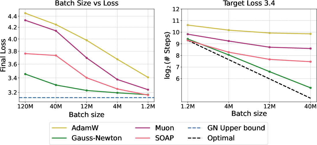
- Full Gauss–Newton reached a target validation loss in 54 steps.
- Layerwise Gauss–Newton did it in 78 steps.
- SOAP needed 292 steps.
- In other words, full Gauss–Newton took about 5.4× fewer steps than SOAP, and layerwise Gauss–Newton was close behind.
- Better scaling to huge batch sizes:
- Gauss–Newton kept improving as the batch size grew, pushing the “critical batch size” much higher than AdamW, Muon, and SOAP.
- This means Gauss–Newton can use bigger batches more effectively, which is great for parallel training on many GPUs.
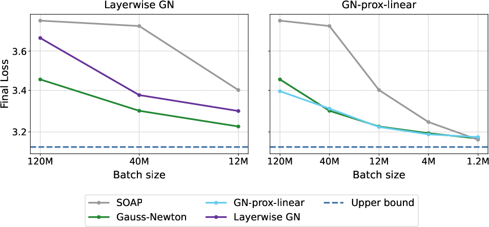
- Layerwise is almost as good as full:
- Even when ignoring cross-layer curvature, the layerwise Gauss–Newton was close to the full method in both steps and final loss.
- That suggests most of the benefit comes from accurate per-layer curvature, not necessarily cross-layer interactions.
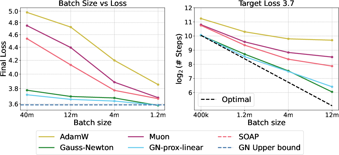
- Extra higher-order loss terms didn’t help much:
- The GN-prox-linear method (which keeps more detailed loss information on a linearized model) performed similarly to Gauss–Newton.
- This implies Gauss–Newton’s approximation is already capturing nearly all the useful curvature for faster convergence.
- There’s a gap between today’s approximations and the “oracle” layerwise method:
- Current practical optimizers (like SOAP and Muon) use efficient approximations. The precise layerwise Gauss–Newton showed that, if we could compute better per-layer curvature, we could get substantially better performance than what’s common today.
Why does this matter?
- Faster training: If we can get close to Gauss–Newton’s performance with practical approximations, LLMs could train in far fewer steps, saving time and energy.
- Better use of big hardware: Gauss–Newton handles very large batches well, which makes it easier to use lots of GPUs in parallel without wasting data or slowing down progress.
- Design direction: The results suggest focusing on:
- Accurate layerwise curvature approximations (since they get most of the gains).
- Smart ways to incorporate Gauss–Newton-like preconditioning without computing giant matrices.
- Reality check: The full method they used is slower per step right now and not production-ready. But it sets a target—an “upper bound” of what’s possible. Future optimizers can aim to get close to this performance while being cheaper to run.
In short, the paper shows that second-order methods—especially Gauss–Newton—have a lot of untapped potential for speeding up LLM training. Most of the benefits can be achieved with layerwise curvature, and there’s room to build more practical algorithms that close the gap with this idealized performance.
Knowledge Gaps
Knowledge gaps, limitations, and open questions
Below is a focused list of open issues the paper leaves unresolved, organized by theme to guide future research.
Scalability and systems considerations
- Scaling to billion-parameter LLMs: The study is limited to 45M–150M parameters; it remains unclear whether the proposed full Gauss-Newton (GN) approach (with JVPs, inner optimization, and line search) remains feasible, stable, and effective for 1B–70B+ models under realistic memory and communication constraints.
- Wall-clock and energy efficiency: Results are reported in iteration complexity and tokens; comprehensive wall-clock time, GPU-hours, throughput, and energy comparisons (including line search and JVP overheads) are missing, especially in multi-node settings with data/model parallelism.
- Memory and communication footprint: The actual memory usage and communication overhead of the GN and layerwise GN implementations are not quantified; practical deployment requires profiling peak memory, activations, and cross-device communication costs.
- Distributed implementation details: No analysis of scalability on large clusters (e.g., DDP/ZeRO, pipeline and tensor parallel); it’s unclear how GN’s inner loops and line search interact with distributed training efficiency and straggler effects.
- Numerical stability and precision: The paper does not report dtype/precision (e.g., bf16/fp8) and numerical stability considerations for JVP/HVP-heavy workloads; robustness under mixed-precision is unknown.
Methodological and theoretical questions
- Inner-solver dependence and accuracy: The method’s performance is tightly coupled to Muon as the inner optimizer; there is no systematic study of inner-solve accuracy (e.g., KKT residuals), stopping criteria, and how solve accuracy trades off with outer-loop convergence.
- “Upper bound” claim validation: The assertion that GN is upper-bounded by Muon with batch size b_inner on the true model is not formally justified under line search and approximation mismatch; provide proofs or counterexamples and quantify empirical gaps to this bound.
- Line search policy and overhead: The choice of line search (candidate step sizes, data used, frequency, stopping conditions) is ad hoc; its compute cost, stability contribution, and sensitivity are not quantified or compared to trust-region/damping alternatives (e.g., Levenberg–Marquardt).
- When do higher-order loss terms matter? GN vs GN-prox-linear appears similar on cross-entropy; it is unknown for other convex losses, non-convex composite objectives, or regimes (e.g., late training) where third/higher-order loss terms might matter; a principled criterion for when to include these terms is missing.
- Spectral and structural analysis: No analysis of curvature spectra, effective condition numbers, or block-structure in attention/MLP to explain why layerwise GN nearly matches full GN; understanding which cross-layer blocks actually matter could inform practical blockwise preconditioners.
- Damping/regularization strategies: The approach uses line search but not systematic damping/trust-region methods; the effect of damping strength, Tikhonov regularization, or LM-style updates on stability and sample efficiency is unexplored.
- Preconditioner variants: Only G{-1} is used; investigating fractional powers (G{-α}), adaptive damping, or hybrid Fisher/GN combinations is left open.
- Convergence guarantees: There are no theoretical guarantees for the outer loop (with inexact inner solves and line search) on non-convex neural objectives; conditions ensuring monotone decrease or global convergence are unaddressed.
Generality across tasks, losses, and architectures
- Beyond language modeling on C4: The study is confined to pretraining on C4; generality to other corpora (code, multilingual, instruction tuning), modalities (vision/speech), or downstream tasks (reasoning, QA, RLHF) is unknown.
- Other loss functions and training regimes: Results hinge on cross-entropy; applicability to other losses (e.g., contrastive, RL objectives), curriculum/mixture-of-objectives, or fine-tuning settings is untested.
- Architectural diversity: Only LLaMA-like transformers (no MoE, long-context models, normalization variants, activation functions) are considered; whether GN gains persist for architectures with different curvature structure is open.
- Sequence length effects: Experiments fix sequence length at 1024; how GN performance and its curvature approximations scale with longer contexts (e.g., 8k–32k) remains unknown.
Batch size scaling and measurement choices
- Mapping “global batch” to practical parallelism: Defining b = N × b_inner (with N inner steps) confounds comparisons with standard large-batch data-parallel training; a principled equivalence between this accumulation scheme and true large minibatches is not established.
- Critical batch size characterization: The study probes up to 120M tokens but does not report uncertainty or sensitivity across seeds; the robustness of critical batch size estimates and the shape of scaling laws (exponents) remain open.
- Early vs late training dynamics: GN’s largest gains appear early; it is unclear how performance evolves in later phases or with much longer training budgets (e.g., tens of billions of tokens).
Fairness, sensitivity, and reproducibility
- Hyperparameter robustness: While sweeps are performed, differences in schedules (e.g., EWA vs cosine) and line-search availability across methods may bias results; a standardized tuning protocol and ablation on schedule choices are needed for fair comparisons.
- Seed variance and confidence intervals: Results are presented without multiple seeds or confidence intervals; variance in iteration counts and final losses should be quantified.
- Code and reproducibility: Implementation details (e.g., exact data for line search, batching policies, autodiff knobs) and code artifacts needed for reproduction at scale are not released or documented.
Alternatives and comparative baselines
- Comparison to Hessian-free CG and K-FAC: The GN method is not directly compared to strong second-order baselines like damped HF+CG or modern K-FAC variants under matched compute; head-to-head wall-clock and sample-efficiency comparisons are missing.
- Specialized solvers for GN-prox-linear: The convex inner problem is solved with Muon; whether specialized convex solvers (e.g., kernel methods, coordinate descent, proximal methods, or second-order convex solvers) yield better accuracy-speed trade-offs is untested.
- Blockwise and hybrid approximations: Between full and layerwise GN, intermediate blockwise schemes (e.g., attention block coupling, QKV tied blocks, residual coupling) are not explored; identifying minimal cross-layer structure needed for near-GN performance is an open design space.
Generalization and implicit bias
- Effects on generalization and calibration: The impact of GN preconditioning on generalization (beyond validation loss), calibration, and robustness is not assessed; implicit bias differences vs first-order methods remain unexplored.
- Overfitting and regularization: Interactions between GN, weight decay, EWA, and other regularizers are not systematically studied; principled regularization for GN (e.g., curvature-aware decay) is open.
Towards new scaling laws and compute-optimality
- Compute-optimal training with second-order methods: Chinchilla scaling is used as a reference, but the compute-optimal batch/sequence/token trade-offs may differ under GN; deriving and validating new scaling laws for second-order-optimized LLMs is an open direction.
- Token efficiency vs step efficiency: A rigorous framework to trade off sample efficiency (tokens) and iteration efficiency (steps), accounting for GN overheads, is needed to judge end-to-end cost-performance at scale.
Glossary
- AdaGrad: An adaptive gradient optimizer that accumulates past squared gradients to adjust per-parameter learning rates. "AdaGrad \citep{JMLR:v12:duchi11a} maintains an accumulator over the vectorized gradient ."
- AdamW: A variant of Adam that decouples weight decay from the gradient-based update to improve generalization. "We run AdamW \citep{adamw}, Muon \citep{jordan2024muon}, and SOAP \citep{vyas2025soapimprovingstabilizingshampoo} as baselines."
- AlgoPerf: A benchmark suite for comparing optimization algorithms across tasks and models. "Shampoo won the recent optimization algorithms benchmark called AlgoPerf \citep{Kasimbeg2025AlgoPerfResults}, outperforming Adam by a margin of 28\%."
- Chinchilla-optimal: Scaling laws that prescribe optimal data and model size trade-offs to maximize performance under a compute budget. "We train 150M-parameter models for 3B tokens following Chinchilla-optimal scaling laws \citep{hoffmann2022trainingcomputeoptimallargelanguage}, ranging batch size from 1.2M to 120M tokens."
- Conjugate gradient (CG): An iterative method for solving large linear systems, often used to approximately compute Newton steps without forming matrices. "prior work on Hessian-free optimizers use the conjugate gradient (CG) to solve an incomplete (unconverged) optimization of the Newton step rather than storing an approximation to the Hessian."
- Critical batch size: The batch size beyond which increasing the batch provides little to no reduction in steps or worsens sample efficiency. "we use a batch size significantly beyond that method's critical batch size \citep{mccandlish2018empiricalmodellargebatchtraining, shallue2019measuringeffectsdataparallelism} such that further increasing batch size does not reduce the number of training steps needed to achieve a given performance."
- Data parallelism: A training paradigm that distributes mini-batches across workers; its efficiency degrades beyond the critical batch size. "We also analyze how this idealized method affects the critical batch size~\citep{mccandlish2018empiricalmodellargebatchtraining, shallue2019measuringeffectsdataparallelism,jain2018parallelizing}, a key measure of data parallelism efficiency."
- Gauss-Newton matrix: A positive semi-definite approximation to the Hessian that captures the curvature of the loss with respect to model outputs while ignoring model curvature. "The Gauss-Newton matrix is defined to be the first term of the following decomposition of the Hessian,"
- GN-prox-linear: A prox-linear variant of Gauss-Newton that minimizes the original convex loss over the linearized model instead of using a second-order loss approximation. "A prox-linear version of Gauss-Newton (GN-prox-linear) \citep{Burke85, drusvyatskiy2017proximalpointmethodrevisited}, which utilizes the higher order information of the loss function itself (see Algorithms~\ref{algorithm:gn} and ~\ref{algorithm:lm} for comparison)."
- Gradient accumulation: A technique to simulate large batch sizes by accumulating gradients over multiple smaller steps before updating parameters. "Since batch sizes are increased using gradient accumulation in our experiments, we choose batch size based on each method's critical batch size to save compute."
- Hessian-free optimization: Second-order optimization that avoids explicitly forming the Hessian by using Hessian-vector products within iterative solvers. "Most related to our work is Hessian-free optimization, which avoids explicit Hessian formation by leveraging Hessian-vector products \citep{hessianfree}."
- Hessian-vector products (HVPs): Products of the Hessian with a vector that enable curvature-aware updates without forming the Hessian. "Most related to our work is Hessian-free optimization, which avoids explicit Hessian formation by leveraging Hessian-vector products \citep{hessianfree}."
- Iteration complexity: The number of optimization steps required to reach a target performance (e.g., a specific validation loss). "we establish a practical upper bound on iteration complexity by applying full Gauss-Newton (GN) preconditioning to transformer models of up to 150M parameters."
- Jacobian-vector products (JVPs): Efficient operations that multiply the Jacobian by a vector, used to compute curvature-related terms without materializing large matrices. "we instead run a functionally equivalent method that leverages Jacobian-vector products (JVPs) to avoid explicitly storing the Hessian."
- Kernelized classification: A framework that uses kernel methods to perform classification in high-dimensional feature spaces induced by kernels. "Moreover, this problem is related to the richly studied literature of kernelized classification \citep{shaikernelclassificatin} (albeit with cross-entropy loss, instead of the max-margin loss)."
- Layerwise Gauss-Newton: A variant that applies Gauss-Newton updates separately per layer, ignoring cross-layer curvature, to reduce computational and memory costs. "Gauss-Newton and Layerwise Gauss-Newton reach the target loss in 54 and 78 steps respectively, compared to 292 steps for SOAP."
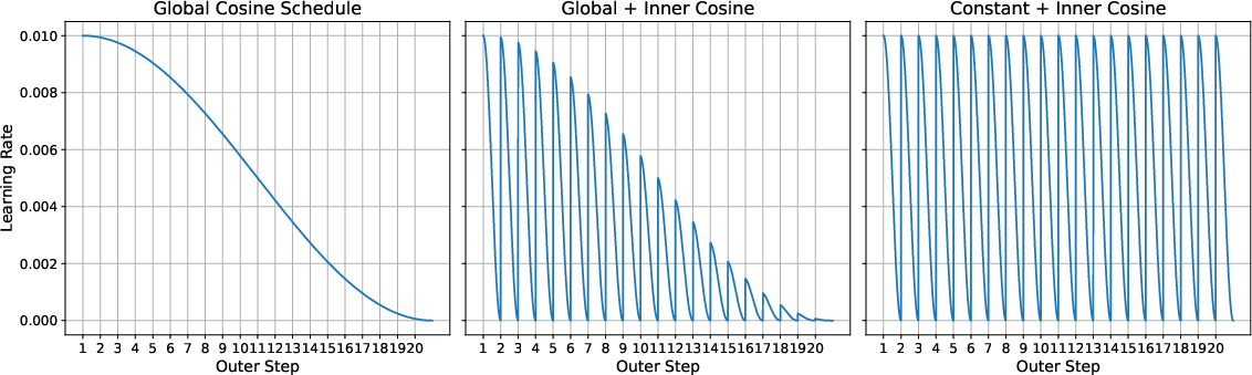
- Learning rate schedules: Prescribed variations of the learning rate over training to improve convergence and stability (e.g., cosine schedules). "We experiment with three learning rate schedules for Gauss-Newton runs, which we refer to as
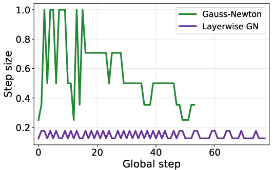
global cosine,''global+inner cosine,'' and ``constant+inner cosine.''" - Line search: A procedure that selects the step size along a proposed update direction by minimizing the loss, improving stability. "We then update the model parameters using a line search."
- Muon: An optimizer that orthonormalizes gradient updates (via Newton-Schulz) and can be viewed as Shampoo without preconditioner accumulation. "Muon \citep{jordan2024muon} tracks the first moment of the gradient, denoted , and performs an orthonormal update:"
- Neural-tangents: A library for computing neural tangent kernels and related Taylor approximations for models. "To compute the necessary Taylor approximations we use the neural-tangents library from \cite{neuraltangents2020}."
- Newton-Schulz orthogonalization procedure: An iterative matrix method used to produce orthonormal updates from gradient information. "where denotes a Newton-Schulz orthogonalization procedure."
- Newton's method: A second-order optimization technique that updates parameters using the inverse Hessian times the gradient. "This is known as Newton's method, and results in the following update rule:"
- Positive semi-definite (PSD): A matrix property where all eigenvalues are non-negative, ensuring well-behaved quadratic forms. "the Hessian is not guaranteed to be positive semi-definite (PSD), and therefore Newton's method does not guarantee that the loss decreases in each iteration or even converges."
- Preconditioner: A matrix or transformation applied to gradients to improve conditioning and accelerate convergence. "Shampoo maintains a separate preconditioner for each dimension of the weight matrix:"
- Shampoo: A second-order optimizer that maintains layerwise left/right preconditioners, approximating Gauss-Newton curvature efficiently. "Shampoo \citep{gupta2018shampoopreconditionedstochastictensor} was originally motivated by AdaGrad, but can be viewed as an approximation of the Gauss-Newton component of the Hessian"
- SOAP: A variant of Shampoo that performs AdamW updates in Shampoo’s eigenbasis to stabilize and improve performance. "SOAP \citep{vyas2025soapimprovingstabilizingshampoo} is a recent variant of Shampoo that runs AdamW \citep{adamw} in the eigenbasis provided by Shampoo."
- Taylor expansion: A local polynomial approximation of a function using its derivatives; used here for first-order model and second-order loss approximations. "be the loss function on the first-order Taylor expansion of around current parameters ."
- Transformer models: Attention-based neural network architectures widely used in LLMs. "applying full Gauss-Newton (GN) preconditioning to transformer models of up to 150M parameters."
- Weight averaging: Exponential moving average of parameters to stabilize training and improve generalization. "For baselines, weight averaging is used only with the constant schedule."
- Weight decay: L2 regularization applied via parameter shrinkage to improve generalization and stability. "we add weight decay to the optimizer as well as a weight decay term to the loss, which adds regularization on the norm of the magnitude of the parameter update."
Practical Applications
Immediate Applications
The following items can be deployed now to improve training workflows, benchmarking, and optimizer selection, with attention to the paper’s empirical results and practical constraints.
- Build a Gauss–Newton “oracle” benchmarking harness for optimizer selection (industry, academia)
- Use full GN and layerwise GN on small-to-mid models (≤150M params) to estimate lower bounds on iteration complexity and critical batch size, then select/tune practical optimizers (e.g., SOAP, Muon) accordingly.
- Potential tools/products/workflows: a “second‑order oracle” suite that runs short GN episodes to rank candidate optimizers and batch sizes; dashboards for iteration/throughput tradeoffs; extensions to AlgoPerf-style benchmarks.
- Assumptions/dependencies: JVP/HVP support in the stack (e.g., JAX/Neural Tangents or equivalent), multiple GPUs, performance ceiling upper-bounded by inner optimizer; results validated on LLaMA-like architectures and C4.
- Plan batch-size scaling and gradient accumulation informed by measured critical batch sizes (industry, cloud training ops)
- Apply findings that AdamW saturates near ~4M tokens, SOAP/Muon ~12–40M, while GN extends further; set gradient accumulation and data-parallel strategies to avoid sample-efficiency loss.
- Potential tools: a “critical batch size estimator” script integrated into MLOps pipelines; automated batch-size schedules tied to validation-loss plateaus.
- Assumptions/dependencies: comparable model/dataset setups; monitoring infrastructure for validation‑loss vs steps; large-batch data loaders.
- Stabilize large-batch training with schedule and line-search strategies distilled from GN runs (software/MLOps)
- Incorporate global cosine or constant+inner cosine schedules, backtracking line search, and warm-starting next inner loop from pre-line-search parameters to reduce instability at large LR.
- Potential tools: optimizer wrappers adding line search and LR schedules; training recipes for SOAP/Muon at large batch sizes.
- Assumptions/dependencies: access to optimizer internals; reliable loss evaluation for line search; telemetry to detect divergence.
- Curvature-aware tuning of layerwise optimizers (software)
- Use the paper’s evidence that precise layerwise curvature captures most GN gains to refine Shampoo/SOAP settings (e.g., preconditioner accumulation, eigenbasis stability, regularization).
- Potential tools: “Shampoo/SOAP curator” that auto-tunes per-layer preconditioners based on curvature proxies; periodic eigenbasis diagnostics.
- Assumptions/dependencies: existing Shampoo/SOAP implementations; telemetry of per-layer gradient statistics; consistency with cross-entropy objectives.
- Fast fine-tuning with few steps on small models (education, startups, research labs)
- Exploit GN/GN‑prox‑linear to push rapid adaptation on ≤150M models for domain-specific corpora when wall-clock costs are acceptable and step count must be minimal.
- Potential tools: JAX-based fine-tuning scripts with GN/GN‑prox‑linear; line-search-enabled trainers for quick convergence.
- Assumptions/dependencies: heavy per-step cost (4–5x), JVP/HVP and line search in stack, cross-entropy tasks; diminishing returns for very large models.
- Extend optimization benchmarks to include “oracle gap” metrics (academia, benchmarking orgs)
- Report the gap between practical methods (e.g., SOAP/Muon) and GN/layerwise GN on standard tasks to set targets for optimizer development.
- Potential tools: expanded AlgoPerf-like benchmark track; public leaderboards with “gap to GN-oracle.”
- Assumptions/dependencies: community adoption, reproducible GN baselines, standard datasets (e.g., C4).
- Training-cost and ESG reporting with optimization-aware projections (policy, enterprise governance)
- Use empirically measured iteration reductions and batch-size scaling behaviors to inform energy/cost projections and procurement decisions emphasizing optimizer R&D.
- Potential tools: cost/energy calculators that incorporate optimizer and batch-size effects; policy briefs on optimization’s role in training efficiency.
- Assumptions/dependencies: mapping iteration changes to energy/wall-clock under current hardware; GN’s per-step overhead may offset step savings.
- Curriculum and methodology for teaching modern second-order methods (academia)
- Incorporate GN, layerwise GN, and GN‑prox‑linear into advanced optimization coursework and labs on LLM training dynamics.
- Potential tools: teaching notebooks; assignments using JVP-based GN to study curvature and critical batch size empirically.
- Assumptions/dependencies: suitable hardware for labs; accessible code (e.g., JAX/Neural Tangents).
Long-Term Applications
The items below require further research, scaling, engineering, or ecosystem development before broad deployment.
- Practical layerwise Gauss–Newton optimizer for billion-parameter LLMs (software, cloud)
- Design a memory/computation‑efficient algorithm that more precisely captures per-layer curvature (approaching the paper’s layerwise oracle) and scales distributedly.
- Potential tools/products: “GN-LLM Trainer” library; PyTorch/JAX kernels for efficient HVP/JVP; distributed line-search modules; cloud managed second‑order optimizer service.
- Assumptions/dependencies: efficient HVP/JVP primitives, numerically stable preconditioners, robust distributed implementations, hardware acceleration.
- Adaptive batch-size schedulers that push the critical batch size upward (cloud training ops)
- Develop curvature-aware controllers that adjust batch size and LR on-the-fly to stay near optimal scaling and minimize sample-efficiency loss.
- Potential products: “Adaptive CBS Scheduler” integrated into training platforms; ML-based controllers trained against GN-oracle targets.
- Assumptions/dependencies: live curvature proxies; reliable loss/gradient telemetry; safe adjustments without destabilizing training.
- Meta-optimization (AutoML for optimizers) using GN-oracle guidance (software/MLOps)
- Use short GN runs to evaluate candidate optimizer configurations, then select per-layer strategies (e.g., Shampoo vs SOAP variants) to minimize the oracle gap.
- Potential tools: optimizer AutoML that searches LR schedules, momentum, preconditioner parameters; CI/CD integration for model training recipes.
- Assumptions/dependencies: compute budget for oracle evaluations; generalization from small-oracle runs to full-scale training.
- Energy- and cost-efficient training policies and standards (policy, consortia)
- Draft procurement guidelines and sustainability standards encouraging adoption of curvature-aware optimization research and reporting of optimizer choices and batch-size scaling.
- Potential outputs: standard metrics for “optimizer efficiency,” reporting templates, incentives for optimization R&D in grants.
- Assumptions/dependencies: large-scale validations; stakeholder buy-in; standardized benchmarking.
- Hardware–software co-design for second-order primitives (semiconductors, cloud)
- Accelerate JVP/HVP and line-search evaluations via specialized kernels or instruction support; rework memory hierarchies to accommodate curvature computations.
- Potential products: GPU/TPU libraries optimized for second-order ops; compiler passes that fuse curvature computations.
- Assumptions/dependencies: vendor collaboration; proven demand from training teams; stability of numerical routines at scale.
- Curvature-informed training curricula and scheduling across phases (LLM training pipelines)
- Integrate second-order phases (e.g., early rapid progress with GN-like steps, then cheaper first-order phases) to reduce total wall-clock while maintaining stability.
- Potential workflows: phased training recipes; automated transitions based on curvature/instability signals.
- Assumptions/dependencies: robust phase-change criteria; consistent gains across datasets/objectives; orchestration support.
- Domain-specific model training acceleration (healthcare, finance, robotics)
- Apply advanced layerwise second-order methods to speed pretraining/fine-tuning of domain LLMs where data and compute are costly, reducing time-to-deployment.
- Potential tools/products: verticalized training services; optimizer presets for medical/financial corpora; rapid compliance documentation enabled by shorter training cycles.
- Assumptions/dependencies: method generalizes beyond C4; domain objectives remain compatible (often cross-entropy-like); privacy/compute constraints.
- Edge/on-device fine-tuning with efficient second-order approximations (mobile/IoT)
- Create compressed, approximate curvature methods enabling small-step adaptation on the edge (e.g., personalization) with limited compute budgets.
- Potential products: lightweight curvature-aware fine-tuning SDKs; hybrid server–edge workflows where server estimates curvature and ships updates.
- Assumptions/dependencies: extreme resource constraints; robust approximations; secure update mechanisms.
Notes on Assumptions and Dependencies Across Applications
- Scalability: Evidence is from 45M–150M param LLaMA models on C4; behavior at billion-scale is promising but unverified.
- Loss/architecture: Results assume cross-entropy with LLaMA-like transformers; other objectives or architectures may differ in PSD properties and curvature behavior.
- Implementation overhead: Full GN is 4–5x slower per step in the study; net wall-clock gains depend on practical approximations approaching the layerwise oracle.
- Inner optimizer dependence: GN performance is upper-bounded by the inner optimizer (Muon in the paper); swapping inner optimizers changes ceilings.
- Stability tooling: Backtracking line search and warm-starting inner loops were critical for stability; productionization requires robust implementations and monitoring.
- Ecosystem: Efficient JVP/HVP and distributed second-order support in mainstream frameworks are prerequisites for broad deployment.
Collections
Sign up for free to add this paper to one or more collections.