Latent Flow Transformer (2505.14513v1)

Abstract: Transformers, the standard implementation for LLMs, typically consist of tens to hundreds of discrete layers. While more layers can lead to better performance, this approach has been challenged as far from efficient, especially given the superiority of continuous layers demonstrated by diffusion and flow-based models for image generation. We propose the Latent Flow Transformer (LFT), which replaces a block of layers with a single learned transport operator trained via flow matching, offering significant compression while maintaining compatibility with the original architecture. Additionally, we address the limitations of existing flow-based methods in \textit{preserving coupling} by introducing the Flow Walking (FW) algorithm. On the Pythia-410M model, LFT trained with flow matching compresses 6 of 24 layers and outperforms directly skipping 2 layers (KL Divergence of LM logits at 0.407 vs. 0.529), demonstrating the feasibility of this design. When trained with FW, LFT further distills 12 layers into one while reducing the KL to 0.736 surpassing that from skipping 3 layers (0.932), significantly narrowing the gap between autoregressive and flow-based generation paradigms.

• The paper introduces Latent Flow Transformer, which compresses multiple transformer layers into one using flow matching techniques.
• It employs a Flow Walking algorithm that refines velocity estimates and ensures accurate transport alignment between latent states.
• Experimental results on the Pythia-410M model demonstrate improved performance and efficient layer distillation compared to traditional baselines.

Latent Flow Transformer: Efficient LLMing via Flow Matching

The paper introduces the Latent Flow Transformer (LFT), a novel architecture designed to improve the parameter and compute efficiency of LLMs by integrating flow-based learning techniques. LFT replaces contiguous blocks of transformer layers with a single learned transport operator, trained via flow matching, thereby compressing the model while maintaining architectural compatibility. Additionally, the paper introduces the Flow Walking (FW) algorithm to address limitations in existing flow-based methods related to preserving coupling between latent states. Experiments on the Pythia-410M model demonstrate that LFT, when trained with FW, can distill multiple layers into one, achieving comparable or superior performance to layer-skipping baselines.

Key Concepts and Methodology

Latent Flow Transformer (LFT) Architecture

The LFT architecture replaces a block of traditional transformer layers with a single latent flow layer. This layer learns a transport operator that @@@@1@@@@ the input latent state at the beginning of the block to the corresponding output latent state using flow-matching principles.

The velocity field estimator $u_\theta(x_t, t)$ is a crucial component of the LFT. The paper uses a transformer layer augmented with scale and shift operators, along with an MLP to predict their factors (Figure 1). The velocity estimate is then derived by subtracting the input latent state from the augmented network's output.

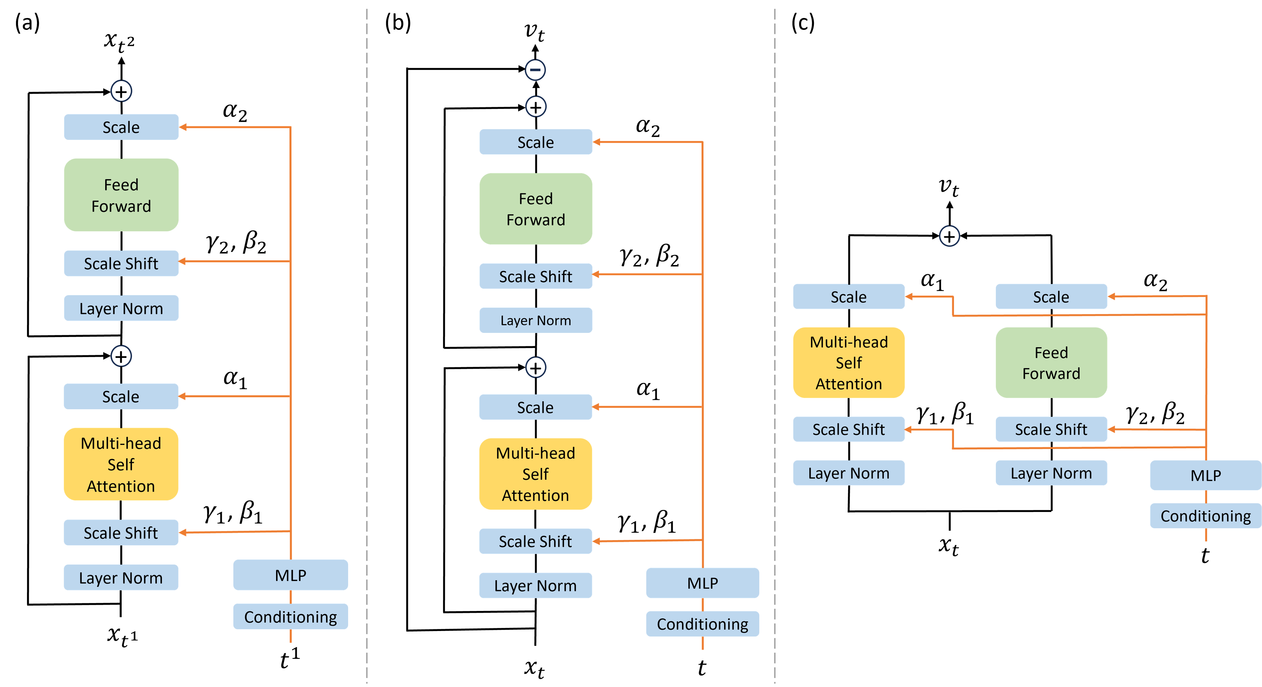
Figure 1: Velocity field estimator architecture details.

Recoupling Ratio for Layer Selection

To determine which blocks of layers are most suitable for replacement, the paper introduces the Recoupling Ratio, an interpretable metric based on Optimal Transport (OT). This metric quantifies the deviation between the original pairing of latent states across layers and the pairing dictated by OT. The OT matrix $M$ represents the ideal pairing between latents at layer $m$ and layer $n$ that minimizes a transport cost, such as Euclidean distance:

$$M = \arg\min_{\gamma} \sum_{i,j} \gamma_{i,j} d(h_m^{(i)}, h_n^{(j)}).$$

The Recoupling Ratio $R$ is defined as:

$$R := 1 - \mathbf{E}\left[\frac{\text{Tr}(M)}{O_M}\right],$$

where $O_M$ is the order of the square matrix $M$. Lower values of $R$ indicate better alignment and fewer flow-crossing issues, making the layer block more suitable for LFT replacement.

Flow Walking (FW) Algorithm

The FW algorithm is introduced to address challenges in flow matching with paired data, where preserving the deterministic correspondence between source and target distributions is critical. FW approximates the mapping from $x_0$ to $x_1$ using numerical integration with discrete time points. The learning of velocity fields is defined by:

$$\mathcal{L}_{\mathrm{FlowWalking}(k)} = \mathbb{E}_{t_{1},\dots,t_{k-1}} \left\|\,x_0 + \sum_{i=1}^k \Delta_{\theta, t_{i}} - x_1\right\|^2,$$

where $$\Delta_{\theta, t_{i}} = s_\theta\bigl(x_{t_{i-1}},\,t_{i-1},t_{i}\bigr) - x_{t_{i-1}}$$, $t_0=0$, $t_k=1$, and $t_i\sim[0,1]$ for $i\in[1,k-1]$. FW learns non-crossing trajectories by slightly separating trajectories around intersecting points, improving transport alignment.

Experimental Results and Analysis

Experimental Setup

The LFT was implemented based on the Pythia-410M model, and experiments were conducted to evaluate layer selection, convergence of flow matching distillations, and inference as an integrated transformer. The evaluation metrics included Normalized Mean Squared Error (NMSE), KL divergence between output $\hat{x}_1$ and target latent $x_1$ ($KL_{x_1||\hat{x}_1}$), empirical KL divergence between the teacher distribution $P$ and the LFT output distribution $Q$ ($KL_{P||Q}$), and perplexity (PPL).

Recoupling Ratio Evaluation

The Recoupling Ratio was computed over different layer choices to assess its ability to predict the feasibility of learning latent flow layers. The results indicated that the Recoupling Ratio aligns with prior observations regarding the qualitatively different transformations applied by early and middle layers in LLMs. Specifically, the early layers exhibited higher Recoupling Ratios, suggesting more flow-crossing issues compared to the middle layers.

Distillation Quality on The Pile

LFTs trained via Standard Flow Matching (LFT-SFM) and Flow Walking (LFT-FW) were compared against layer-skipping and regression baselines. The models were trained on 2.6 billion tokens from The Pile dataset, replacing either layers 6-12 or layers 6-18 of Pythia-410m with a single flow-matching layer.

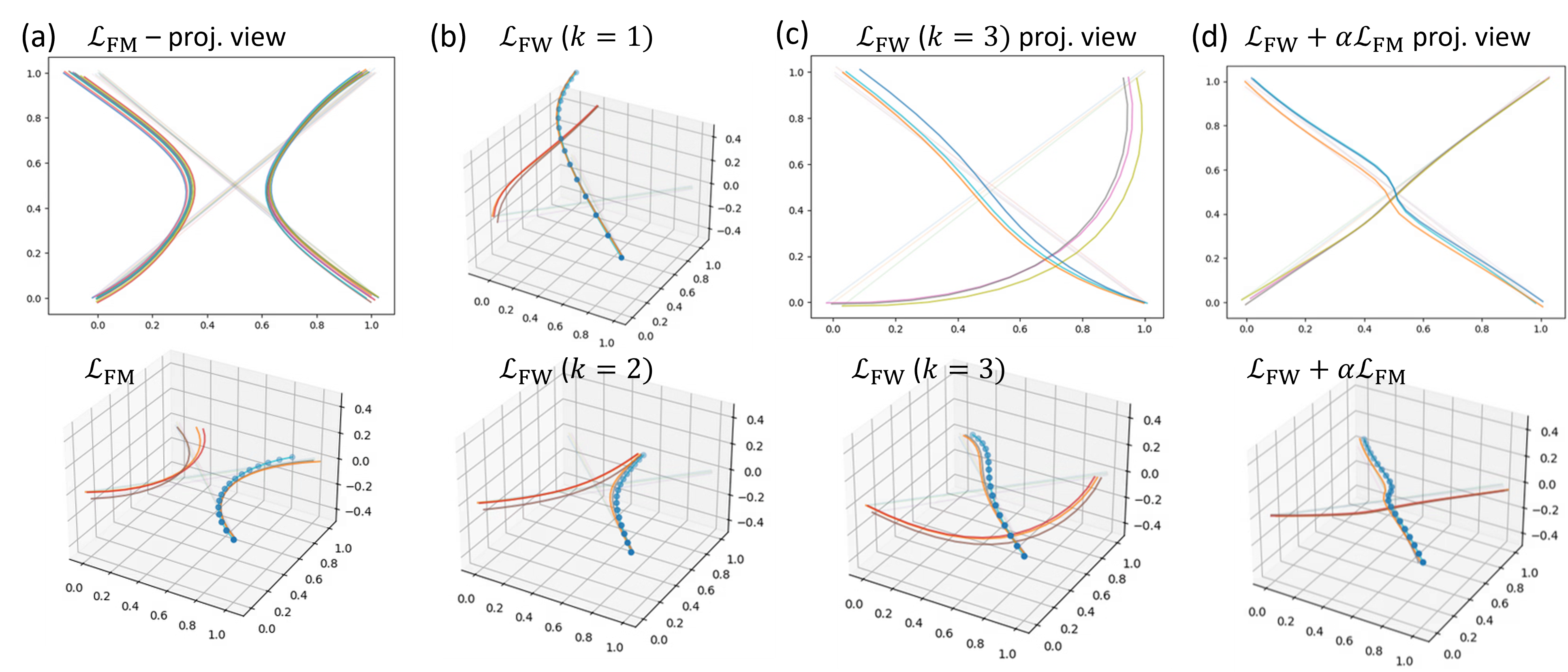
Figure 2: Paired flow matching trajectories.

The results showed that both LFT-SFM and LFT-FW converged rapidly and outperformed naive layer-skipping. LFT-FW consistently outperformed both baselines in terms of latent-state matching and downstream LLMing. For instance, LFT-FW with $k=1$ achieved parity with the regression model and outperformed LFT-SFM with $k=8$, indicating that FW's implicit velocity estimates more accurately guide the model toward its target hidden state.

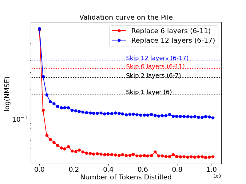
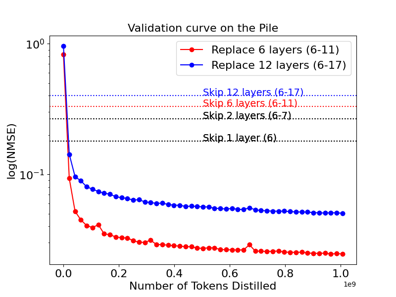
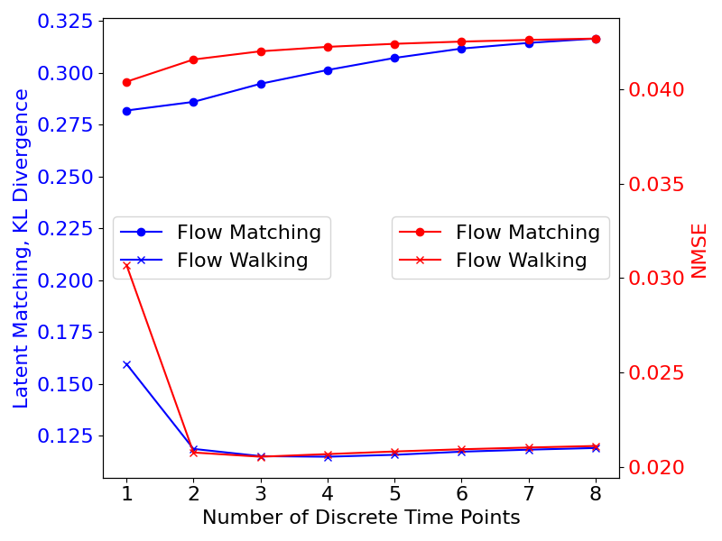
Figure 3: LFT trained with flow matching vs layer-skipping baselines.

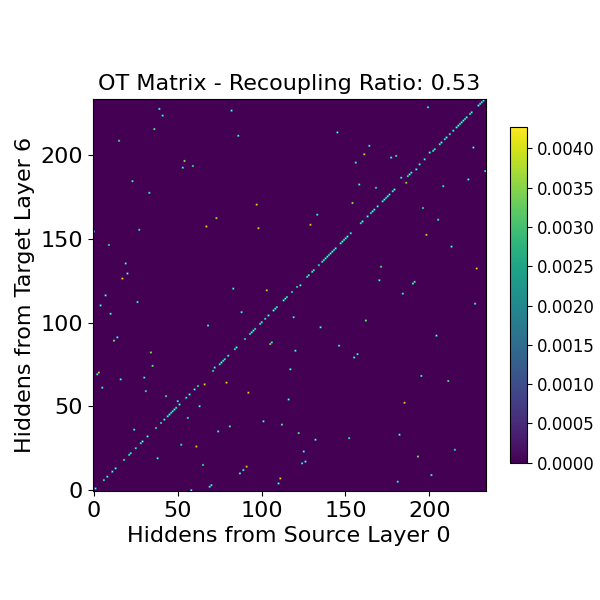
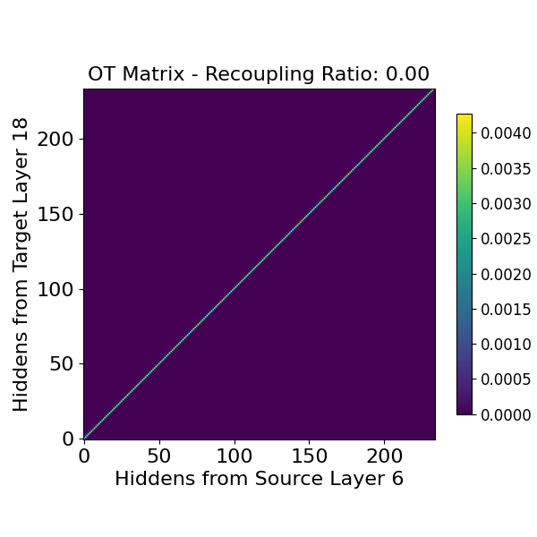
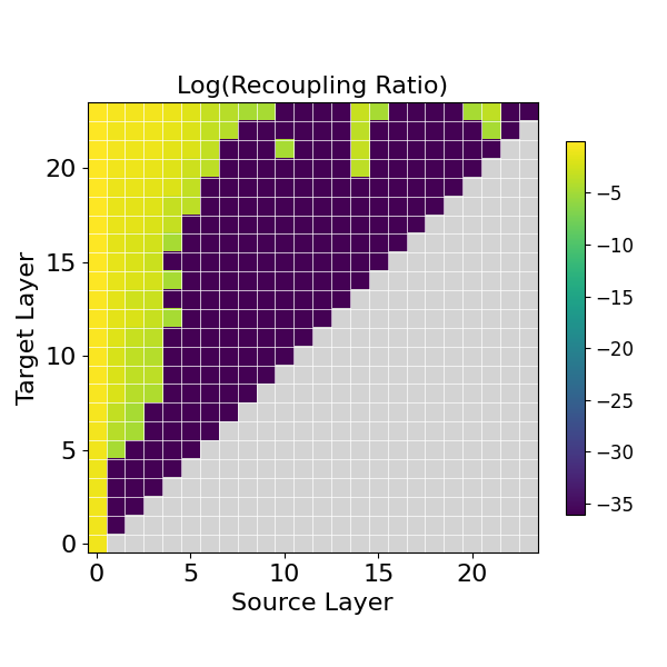
Figure 4: OT matrix of paired hiddens between layer 0 and layer 6.

Effect of Discrete Time Points on Inference

The number of discrete time points $k$ was identified as a key hyperparameter during inference. For LFT-SFM, decreasing $k$ reduced both KL divergence and NMSE, suggesting that early velocity estimates more accurately steer the hidden state. LFT-FW achieved optimal performance at $k=3$, corresponding to the three-step integration in the FW algorithm.

Implications and Future Directions

The LFT architecture, combined with the FW algorithm, presents a promising approach for compressing and accelerating LLMs. By replacing multiple transformer layers with a single learned transport operator, LFT reduces the parameter count and computational complexity while maintaining or improving performance. The Recoupling Ratio offers a valuable tool for identifying compressible layer blocks within transformer models.

Future research directions include:

• Optimizing input and output layers to minimize flow crossing.
• Exploring architectural search and initialization methods for flow-replaced transformers.
• Scaling up experiments to larger models and datasets.
• Training flow-replaced transformers from scratch without pretraining.

Conclusion

The Latent Flow Transformer represents a significant step toward more efficient and scalable LLMs. By leveraging flow-matching principles and introducing the Flow Walking algorithm, this research effectively bridges the gap between autoregressive and flow-based modeling paradigms, offering a pathway to substantial parameter reduction and improved inference performance. The empirical results on the Pythia-410M model validate the feasibility and potential of the LFT architecture for future LLM development.