MVSNet: Depth Inference for Unstructured Multi-view Stereo

Abstract: We present an end-to-end deep learning architecture for depth map inference from multi-view images. In the network, we first extract deep visual image features, and then build the 3D cost volume upon the reference camera frustum via the differentiable homography warping. Next, we apply 3D convolutions to regularize and regress the initial depth map, which is then refined with the reference image to generate the final output. Our framework flexibly adapts arbitrary N-view inputs using a variance-based cost metric that maps multiple features into one cost feature. The proposed MVSNet is demonstrated on the large-scale indoor DTU dataset. With simple post-processing, our method not only significantly outperforms previous state-of-the-arts, but also is several times faster in runtime. We also evaluate MVSNet on the complex outdoor Tanks and Temples dataset, where our method ranks first before April 18, 2018 without any fine-tuning, showing the strong generalization ability of MVSNet.

• The paper introduces an end-to-end deep learning architecture that extracts deep image features and constructs a 3D cost volume for multi-view stereo reconstruction.
• It employs differentiable homography warping and a variance-based cost metric to fuse features from arbitrary N-view images for robust depth inference.
• The framework integrates a depth residual learning network for refinement, achieving superior performance on the DTU and Tanks and Temples datasets.

MVSNet: Depth Inference for Unstructured Multi-view Stereo

MVSNet is an end-to-end deep learning architecture designed for depth map inference from multi-view images. The network extracts deep visual image features and constructs a 3D cost volume via differentiable homography warping. 3D convolutions are then applied for regularization and initial depth map regression, followed by refinement using the reference image. The framework uses a variance-based cost metric to handle arbitrary N-view inputs. MVSNet demonstrates state-of-the-art performance on the DTU dataset and strong generalization on the Tanks and Temples dataset (1804.02505).

Network Architecture

The MVSNet architecture (Figure 1) comprises several key components that facilitate depth map inference from multiple views.

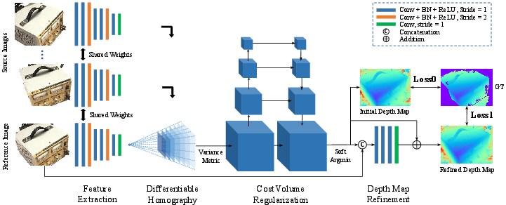
Figure 1: The network design of MVSNet, illustrating the 2D feature extraction, differentiable homography warping, cost volume regularization, and depth map refinement stages.

Image Feature Extraction

Initial processing involves extracting deep features $\{\mathbf{F}_i\}_{i=1}^{N}$ from $N$ input images $\{\mathbf{I}_i\}_{i=1}^{N}$ using an eight-layer 2D CNN. Strides in specific layers create a multi-scale feature representation, with each convolutional layer followed by batch normalization (BN) and a rectified linear unit (ReLU), except for the final layer. Parameters are shared across feature towers to enhance learning efficiency. This process yields $N$ 32-channel feature maps, downsized by a factor of four in each dimension.

Cost Volume Construction

Following feature extraction, a 3D cost volume is constructed upon the reference camera frustum. The differentiable homography operation warps feature maps into different fronto-parallel planes relative to the reference camera, forming $N$ feature volumes $\{\mathbf{V}_i\}_{i=1}^N$. The homography $\mathbf{H}_i(d)$ between the $i^{th}$ feature map and the reference feature map at depth $d$ is defined as:

$$\mathbf{H}_i(d) = \mathbf{K}_i \cdot \mathbf{R}_i \cdot \Big(\mathbf{I} - \frac{(\mathbf{t}_1 - \mathbf{t}_i) \cdot \mathbf{n}_1^T}{d} \Big) \cdot \mathbf{R}_1^T \cdot \mathbf{K}_1^T$$

where $\mathbf{K}_i$, $\mathbf{R}_i$, and $\mathbf{t}_i$ represent the camera intrinsics, rotations, and translations, respectively, and $\mathbf{n}_1$ is the principal axis of the reference camera.

A variance-based cost metric $\mathcal{M}$ then aggregates the feature volumes $\{\mathbf{V}_i\}_{i=1}^N$ into a single cost volume $\mathbf{C}$, expressed as:

$\mathbf{C} = \mathcal{M}(\mathbf{V}_1, \cdots, \mathbf{V}_N) = \frac{\sum\limits_{i=1}^N{(\mathbf{V}_i - {\mathbf{V}_i})^2}{N}$

where ${\mathbf{V}_i}$ is the average volume among all feature volumes.

Cost Volume Regularization and Depth Map Estimation

Multi-scale 3D CNNs, similar to a 3D UNet, regularize the cost volume $\mathbf{C}$ to generate a probability volume $\mathbf{P}$. This network refines the cost volume using an encoder-decoder structure, aggregating information from a large receptive field. The final convolutional layer outputs a 1-channel volume, and the softmax operation is applied along the depth direction for probability normalization. The depth map $\mathbf{D}$ is then estimated by computing the expectation value along the depth direction:

$\mathbf{D} = \sum\limits_{d=d_{min}^{d_{max} d \times \mathbf{P}(d)$

This operation approximates the argmax result and produces a continuous depth estimation. The probability map, derived from the probability distribution along the depth direction, reflects the depth estimation quality.

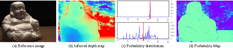
Figure 2: Illustrations of the inferred depth map, probability distributions, and probability map, highlighting the relationship between probability distribution and depth estimation quality.

Depth Map Refinement

A depth residual learning network refines the initial depth map using the reference image as a guide. The initial depth map and the resized reference image are concatenated and passed through a series of 2D convolutional layers to learn the depth residual, which is then added back to refine the depth map.

Training and Implementation Details

Data Preparation and View Selection

The DTU dataset [aanaes2016large] is used for training, where ground truth depth maps are generated from provided point clouds using screened Poisson surface reconstruction (SPSR) [kazhdan2013screened]. A reference image and two source images ($N=3$) are selected based on a scoring function that favors a baseline angle $\theta_0$:

$$\mathcal{G}(\theta) = \left\{ \begin{array}{ll} \exp(-\frac{(\theta - \theta_0)^2}{2\sigma_1^2}), \theta \leq \theta_0 \ \exp(-\frac{(\theta - \theta_0)^2}{2\sigma_2^2}), \theta > \theta_0 \ \end{array} \right.$$

Images are downsized and cropped to $640 \times 512$ for training, with depth hypotheses uniformly sampled from $425mm$ to $935mm$ with a $2mm$ resolution ($D=256$).

Loss Function

The training loss is the mean absolute difference between the ground truth depth map and the estimated depth map:

$Loss = \sum\limits_{p \in \mathbf{p}_{valid} \underbrace{\| d(p) - \hat{d_{i}(p) \|_1}_{Loss0} + \lambda \cdot \underbrace{\| d(p) - \hat{d_{r}(p) \|_1}_{Loss1}$

where $\mathbf{p}_{valid}$ denotes valid ground truth pixels, $d(p)$ is the ground truth depth value, $\hat{d_{i}(p)$ is the initial depth estimation, and $\hat{d_{r}(p)$ is the refined depth estimation.

Post-Processing and Depth Map Fusion

Post-processing involves depth map filtering based on photometric and geometric consistencies. Photometric consistency uses the probability map, while geometric consistency ensures depth consistency among multiple views. A visibility-based fusion algorithm integrates depth maps from different views into a unified point cloud representation.

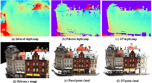
Figure 3: Reconstructions of scan 9 from the DTU dataset, illustrating the depth map, filtered depth map, ground truth depth map, reference image, fused point cloud, and ground truth point cloud.

Experimental Results

DTU Dataset

On the DTU dataset [aanaes2016large], MVSNet outperforms existing methods in completeness and overall quality, achieving superior results in textureless and reflective areas. Quantitative results on the DTU evaluation set are shown in Table 1.

Tanks and Temples Dataset

MVSNet demonstrates strong generalization on the Tanks and Temples dataset [knapitsch2017tanks], ranking first among submissions before April 18, 2018, without any fine-tuning. This highlights the network's ability to generalize to complex outdoor scenes. Qualitative point cloud results of the intermediate set are shown in Figure 4.

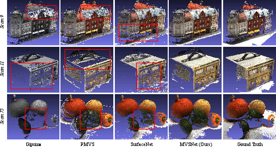
Figure 5: Qualitative results on the DTU dataset, showcasing the completeness of MVSNet in textureless and reflective areas.

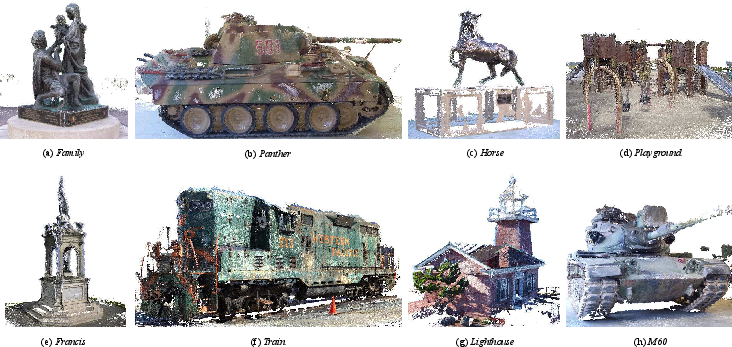
Figure 4: Point cloud results on the Tanks and Temples dataset, demonstrating the generalization ability of MVSNet on complex outdoor scenes.

Ablation Studies

Ablation studies validate the contribution of individual components. Increasing the input view number $N$ reduces the validation loss. The learning-based image feature extraction significantly boosts reconstruction quality compared to using a single convolutional layer. The variance-based cost metric converges faster with lower validation loss than the mean operation-based metric. The depth refinement network also improves evaluation results. Ablation studies are summarized in Figure 6.

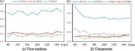
Figure 6: Results of ablation studies, showing the impact of view numbers, image features, cost metric, and depth map refinement on validation loss.

Conclusion

MVSNet introduces an end-to-end deep learning architecture for MVS reconstruction, leveraging differentiable homography to build cost volumes and demonstrating state-of-the-art performance and generalization capabilities (1804.02505). Future work may focus on refining training data and exploring alternative network architectures to further improve reconstruction quality and efficiency.