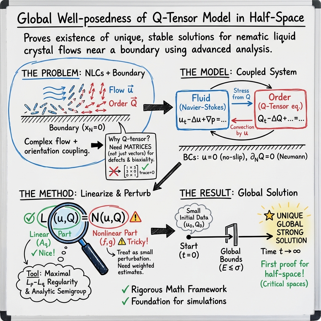
Q-Tensor Model of Nematic Liquid Crystals

• The Q-tensor model is a continuum, tensorial framework that quantifies nematic liquid crystal order by capturing both the magnitude and anisotropy of molecular alignment.
• It couples the Navier–Stokes equations with a relaxational PDE for the Q-tensor, derived from the Landau–de Gennes free energy, to analyze defect structures and phase transitions.
• Global well-posedness in a half-space is established using maximal Lp–Lq regularity and analytic semigroup methods under small initial data conditions.

A Q-tensor model of nematic liquid crystals is a continuum, tensorial framework for describing the orientational order and hydrodynamics of nematic phases. In the Q-tensor formalism, the order parameter is a symmetric traceless matrix field $Q(x,t)\in S_0^{N}$, which captures both the magnitude and the anisotropy of the molecular alignment, including both uniaxial and biaxial states. The Q-tensor model couples the Navier–Stokes equations for incompressible flow to a parabolic or relaxational partial differential equation (PDE) for $Q$, typically derived from the Landau–de Gennes free energy. This approach encompasses the full Beris–Edwards hydrodynamic theory, enabling the description of rich defect structures, flows, and phase transitions inaccessible to vector-based director models.

1. Mathematical Formulation of the Q-Tensor Model

The Beris–Edwards Q-tensor model describes the evolution of the velocity field $u:\mathbb{R}^N_+\times\mathbb{R}_+\to\mathbb{R}^N$, pressure $p:\mathbb{R}^N_+\times\mathbb{R}_+\to\mathbb{R}$, and Q-tensor field $Q:\mathbb{R}^N_+\times\mathbb{R}_+\to S_0^N$ (the space of symmetric, traceless $N\times N$ matrices). The system, posed in the half-space $\mathbb{R}^N_+=\{x=(x',x_N): x_N>0\}$, is

$$\begin{aligned} & u_t + (u\cdot\nabla)u + \nabla p = \Delta u + \operatorname{div}[\tau(Q)+\sigma(Q)], \quad \nabla\cdot u = 0, \ & Q_t + (u\cdot\nabla)Q - S(\nabla u,Q) = - H(Q), \end{aligned}$$

with constitutive and energetic definitions:

• Symmetric and antisymmetric velocity gradients: $D(u)=\frac12(\nabla u + (\nabla u)^T)$, $\Omega(u)=\frac12(\nabla u - (\nabla u)^T)$.
• Landau–de Gennes free energy

$$\mathcal{F}(Q) = \int_{\mathbb{R}^N_+} \Big[ \frac12|\nabla Q|^2 + \tfrac12 a\, \operatorname{tr}Q^2 - \tfrac13 b\, \operatorname{tr}Q^3 + \tfrac14 c\, (\operatorname{tr}Q^2)^2 \Big] dx,$$

with material constants $a,b,c$.

• Molecular field (variational derivative)

$$H(Q) = \Delta Q - aQ + b \big(Q^2 - (\operatorname{tr}Q^2)/N\, I \big) - c Q\, \operatorname{tr} Q^2.$$

• Co-rotational coupling

$$S(\nabla u,Q) = (\xi D(u) + \Omega(u))(Q + I/N) + (Q + I/N)(\xi D(u) - \Omega(u)) - 2\xi (Q + I/N) \operatorname{tr}(Q \nabla u).$$

• Extra stress tensors:

$$\begin{aligned} \tau(Q) &= 2\xi\, \operatorname{tr} Q (Q+I/N) - \xi \left[ (Q+I/N)^2 + (Q+I/N)^2 \right] - \nabla Q \odot \nabla Q, \ \sigma(Q) &= -Q H(Q) + H(Q) Q, \end{aligned}$$

where $$(\nabla Q\odot\nabla Q)_{ij} = \sum_{k\ell} \partial_i Q_{k\ell}\, \partial_j Q_{k\ell}$$.

Boundary and initial conditions specified on the half-space are:

• No-slip for the velocity and homogeneous Neumann for $Q$ at $x_N=0$: $u|_{x_N=0}=0$, $\partial_{N} Q|_{x_N=0}=0$.
• Prescribed initial data: $u(x,0)=u_0(x)$, $Q(x,0)=Q_0(x)$.

2. Functional Setting and Operator Framework

The analysis is conducted in the $L_p$-$L_q$ maximal regularity framework. Key spaces are:

• Solenoidal velocity space: $J_q(\mathbb{R}^N_+)=\overline{C^\infty_0}^{L^q}$ of divergence-free vector fields.
• Pressure and tensor spaces: $\dot{H}^1_{q,0}(\mathbb{R}^N_+)$ for $Q$, incorporating boundary/trace constraints.

The coupled system is rewritten in a perturbative form introducing $\beta=2\xi/N$, separating linear and nonlinear contributions: $$\begin{aligned} & u_t - \Delta u + \nabla p + \beta (\Delta Q - a Q) = f(u,Q), \ & Q_t - \beta\, \operatorname{div} u - \Delta Q + aQ = g(u,Q), \end{aligned}$$ where $f,g$ are quadratic and higher-order nonlinearities depending on $(u,Q)$. The principal linear operator

$$A_q(u,Q) = (-\Delta u + \nabla K(u,Q) - \beta(\Delta Q - aQ),\; \beta\,\operatorname{div} u + \Delta Q - aQ)$$

acting on $(u,Q)\in J_q \times \dot{H}^1_q$ admits crucial properties:

• Analytic semigroup generation: $A_q$ generates an analytic semigroup on $X_q=J_q\times\dot{H}^1_q$.
• Maximal $L_p$-$L_q$ regularity: The associated resolvent problem exhibits $\mathcal{R}$-boundedness, enabling full scale-invariant regularity estimates.

3. Global Well-posedness and Main Results

For $N\ge2$, $0<\theta<1/2$, and suitable exponents $(q_0,q_1,q_2,p)$ tied to $\theta$ by

$$1/q_0=(1+2\theta)/N,\quad 1/q_1=(1+\theta)/N,\quad 1/q_2=\theta/N,\quad 1/p<\theta/2,$$

the main theorem establishes:

If the initial data $(u_0,Q_0)$ lie in the intersection of the appropriate regularity class and are sufficiently small, i.e. $$> \sum_{i=1}^2 \|(u_0,Q_0)\|_{X_{q_i,p}} + \|(u_0,Q_0)\|_{J_{q_0}\times\dot{H}^1_{q_0}} \le \sigma^2, >$$ with $\sigma>0$ sufficiently small, then the nonlinear Q-tensor system admits a unique global solution $(u,Q,p)$ in $$> \begin{aligned} > & u_t,\ \nabla^2 u\in L_p(\mathbb{R}_+; L_{q_i}(\mathbb{R}^N_+)),\ > & u\in L_p(\mathbb{R}_+; H^2_{q_i}),\quad Q_t\in L_p(\mathbb{R}_+; H^1_{q_i}),\ > & Q\in L_p(\mathbb{R}_+; H^3_{q_i}\cap H^1_{q_i}),\quad \nabla p\in L_p(\mathbb{R}_+; L_{q_i}), > \end{aligned} >$$ for $i=1,2$, and satisfies the global a-priori bound $$> E(u,Q):=\sum_{i=1}^2 \Bigl[ \|(1+t)(u_t,\nabla^2 u)\|_{L_pL_{q_i}} + \|(1+t)\nabla Q\|_{L_pL_{q_i}} + \|(u,Q)\|_{L_pX_{q_i}} + \|(u,Q)\|_{L_\infty X_{q_i}} \Bigr] \leq \sigma. >$$

This result confirms the first unique global-in-time strong solution for the Q-tensor model in the half-space, under sharp smallness conditions and in critical function spaces.

4. Key Analytical Ingredients and Estimates

The proof employs several advanced tools from modern PDE theory:

• Maximal $L_p$-$L_q$ regularity for the linearized system, anchored in the $\mathcal{R}$-boundedness of the resolvent and analytic semigroup theory (Theorem 3.1).
• Weighted-in-time estimates—by a differentiation in time of the semigroup, yielding bounds for $(1+t)(u_t,\nabla^2 u,Q_t)$.
• Nonlinear contraction—embedding, Gagliardo–Nirenberg, and interpolation inequalities ensure the nonlinear map taking $(u,Q)$ to the solution of the linear system with right-hand side $(f(u,Q),g(u,Q))$ is a contraction on the small ball defined by $E(u,Q)\leq \sigma$.

Central estimates include:

• Maximal regularity (Theorem 3.1, Eq. 3.5):

$$\|(u_t,\nabla^2 u,Q_t,\nabla Q)\|_{L_p(\mathbb{R}_+; L_q\times\dot H^1_q)} + \|\nabla p\|_{L_p(\mathbb{R}_+; L_q)} \leq C\left(\|(u_0,Q_0)\|_{X_{q,p}} + \|(f,g)\|_{L_p(\mathbb{R}_+; L_q)}\right)$$

• Weighted bound (Theorem 4.1):

$$\|(1+t)(u_t,\nabla^2u,Q_t,\nabla Q)\|_{L_p(\mathbb{R}_+;L_q\times\dot H^1_q)} + \|(u,Q)\|_{L_\infty(\mathbb{R}_+; \dot H^{0,1}_q)} \leq C\left(\|(u_0,Q_0)\|_{X_{q,p}} + \|(1+t)(f,g)\|_{L_pL_q} + \text{l.o.t.}\right)$$

• Nonlinearity control (Eq. 5.7):

$$\sum_{r\in\{q_0,q_1,q_2\}}\|(1+t)(f(u,Q),g(u,Q))\|_{L_pL_r} \leq C\sum_{k=2}^5 E(u,Q)^k,$$

enabling control via smallness of $E(u,Q)$. The Banach fixed-point argument concludes the existence and uniqueness.

5. Boundary, Initial Conditions, and Physical Interpretation

The boundary conditions specify complete anchoring for velocity (no-slip), $u|_{x_N=0}=0$, and homogeneous Neumann (natural) conditions for $Q$, $\partial_N Q|_{x_N=0}=0$, modeling a flat substrate enforcing zero flow and free orientational relaxation. Initial conditions require $(u_0,Q_0)\in$ intersection of scale-invariant $L_p$–$L_q$ spaces and their traces.

Physically, this setup models the hydrodynamics of nematic liquid crystals in the presence of a rigid boundary, capturing defect relaxation, flow-alignment effects, and nonlinear coupling between the velocity and orientational order, within the small-data regime ensuring global regularity.

6. Comparison to Prior Results and Analytical Significance

This result establishes the global well-posedness for the full Beris–Edwards Q-tensor model in the half-space under critical regularity and scaling. It extends earlier global well-posedness results in bounded domains and in $\mathbb{R}^N$ for small initial data (see Xiao (Xiao, 2016), Murata–Shibata (Murata et al., 2021)), resolving the technical challenge posed by the presence of a boundary and nontrivial coupling through Dirichlet–Neumann formulations. The proof synthesizes maximal regularity, semigroup decay, and nonlinear contraction in a Banach space, and refines all relevant linear and nonlinear analysis in the presence of a boundary.

The approach is robust and admits immediate adaptation to related coupled flow–order parameter systems, provided their linearization admits suitable $\mathcal{R}$-boundedness and semigroup properties.

7. Implementation and Extension Considerations

Implementation of the Q-tensor model in the half-space requires discretization strategies compatible with the imposed boundary conditions for $(u,Q)$ and the structure of the stress terms. The well-posedness theory justifies the use of time-stepping and spatial discretizations (finite element, spectral, or finite difference) in critical $L_p$-$L_q$ settings, with the regularity results ensuring numerical stability for small data.

For physical and computational models targeting the defect-rich, nonlinear regime, further developments are required to address potential blow-up or singularity formation for large data. However, the analytic framework developed provides a blueprint for the paper of Q-tensor models in unbounded and semi-infinite domains, as well as for the incorporation of additional physical effects (temperature variation, electric fields, surface anchoring, etc.) provided the structure of the nonlinearities and boundary conditions allows analogous maximal-regularity and fixed-point strategies.