Wasserstein-Cramér-Rao Theory of Unbiased Estimation
Abstract: The quantity of interest in the classical Cramér-Rao theory of unbiased estimation (e.g., the Cramér-Rao lower bound, its exact attainment for exponential families, and asymptotic efficiency of maximum likelihood estimation) is the variance, which represents the instability of an estimator when its value is compared to the value for an independently-sampled data set from the same distribution. In this paper we are interested in a quantity which represents the instability of an estimator when its value is compared to the value for an infinitesimal additive perturbation of the original data set; we refer to this as the "sensitivity" of an estimator. The resulting theory of sensitivity is based on the Wasserstein geometry in the same way that the classical theory of variance is based on the Fisher-Rao (equivalently, Hellinger) geometry, and this insight allows us to determine a collection of results which are analogous to the classical case: a Wasserstein-Cramér-Rao lower bound for the sensitivity of any unbiased estimator, a characterization of models in which there exist unbiased estimators achieving the lower bound exactly, and some concrete results that show that the Wasserstein projection estimator achieves the lower bound asymptotically. We use these results to treat many statistical examples, sometimes revealing new optimality properties for existing estimators and other times revealing entirely new estimators.
Paper Prompts
Sign up for free to create and run prompts on this paper using GPT-5.
Top Community Prompts
Explain it Like I'm 14
Overview
This paper looks at a new way to judge how “stable” a statistical estimator is. In classical statistics, we often ask: “If I took another, independent sample, how much would my estimator change?” That change is measured by variance. This paper instead asks: “If I make a tiny, smooth tweak to the same data (like adding a tiny bit of noise), how much does the estimator change?” That change is called sensitivity.
The authors build a full theory around sensitivity that closely mirrors the famous Cramér–Rao theory for variance. They create sensitivity versions of:
- A universal lower bound (the best possible you can ever do),
- The types of models where that bound can be reached exactly,
- An estimator that reaches the bound asymptotically (with lots of data).
Key Questions
The paper focuses on three simple questions:
- How small can the sensitivity of an unbiased estimator be?
- For which statistical models is it possible to exactly achieve that smallest sensitivity?
- Is there a general-purpose estimator that (at least asymptotically) achieves that optimal sensitivity?
How Did They Study It? Key Ideas and Analogies
To make these ideas accessible, here are the main concepts with simple analogies:
- Unbiased estimator: An estimator is unbiased if, on average, it gets the right answer. Think of guessing the average height of students; if your method averages out to the true average over many tries, it’s unbiased.
- Variance vs. sensitivity:
- Variance: How much your estimate changes if you redo the entire experiment with fresh, independent data.
- Sensitivity: How much your estimate changes if you add tiny, random nudges (noise) to the same data points. This captures how fragile your estimator is to small measurement errors.
- Two “geometries” on the space of probability distributions:
- Fisher–Rao/Hellinger geometry (classical): Measures instability through variance. It’s like reweighting the distribution (changing how much each outcome counts).
- Wasserstein geometry (new focus): Measures instability through sensitivity. It’s like moving mass in a “sand pile.” Imagine a probability distribution as a pile of sand; the Wasserstein distance measures how far you have to move the sand to reshape one pile into another.
- Optimal transport and Wasserstein distance: Optimal transport finds the most efficient way to move the “sand” (probability mass) from one shape to another. The Wasserstein distance is the total “work” required. This geometry naturally captures how small perturbations of data move the distribution.
- Differentiability in the Wasserstein sense (DWS): This is a smoothness condition on a statistical model: as the parameter changes a tiny bit, the optimal transport map (the way mass moves) also changes smoothly. It’s the sensitivity-world version of a standard smoothness condition (DQM) used in the variance-world.
- Wasserstein information, J(θ): A number (or matrix in higher dimensions) that captures how sensitive the distribution is to tiny changes in its parameter, within the Wasserstein framework. It plays the same role as Fisher information in the variance framework.
- Wasserstein–Cramér–Rao (WCR) lower bound: A fundamental inequality saying sensitivity cannot go below a certain level. In simple terms:
- Sensitivity ≥ constant × 1/n,
- Where the constant depends on the estimand (the thing you want to estimate) and the Wasserstein information J(θ).
- In symbols (one-parameter case): Sen ≥ (χ′(θ))² / (n J(θ)).
- This mirrors the classical Cramér–Rao bound for variance.
- Transport families (analogy to exponential families): These are special models where the way mass moves (under optimal transport) has a neat structure. In such models, the authors show you can build unbiased estimators that exactly achieve the WCR bound—just like exponential families in classical statistics allow exact attainment of the classical Cramér–Rao bound.
- Wasserstein Projection Estimator (WPE): An estimator that fits your model to the empirical data by minimizing the Wasserstein distance between the model and the observed data distribution. Think: “Find the parameter whose model ‘sand pile’ is closest to the data ‘sand pile’.” This is analogous to the Maximum Likelihood Estimator (MLE), which fits the model using Kullback–Leibler divergence instead. The authors show WPE is asymptotically sensitivity-efficient under suitable conditions.
Main Findings and Why They Matter
Here are the main results, explained with examples and reasons they matter:
- A universal lower bound for sensitivity (WCR bound):
- No unbiased estimator can have sensitivity smaller than the WCR bound. This gives a target to aim for and a benchmark to compare estimators.
- Importance: Just like the classical Cramér–Rao bound for variance sets a limit, the WCR bound sets the limit for design of stable estimators under measurement noise.
- Exact efficiency in transport families:
- The authors define “transport families” (models with a special optimal transport structure) and prove that in these families, there exist unbiased estimators that exactly hit the WCR bound.
- Importance: This tells you when perfect sensitivity performance is achievable and how to construct such estimators.
- The WPE reaches the bound asymptotically:
- The Wasserstein Projection Estimator (WPE) is shown to be asymptotically sensitivity-efficient. In large samples, it gets as close as possible to the lower bound.
- Importance: WPE offers a general, practical way to design estimators that are stable to small noise.
- Concrete examples (why estimators behave differently under sensitivity than variance):
- Gaussian mean:
- Sample mean is optimal for both variance and sensitivity: Var ~ 1/n, Sensitivity ~ 1/n.
- Reason: Averaging spreads the effect of noise, causing lots of cancellations.
- Uniform [0, θ] scale:
- MLE = max(X) has tiny variance (~1/n²) but large, non-shrinking sensitivity (constant order).
- A linear estimator (twice the mean) has variance ~ 1/n and sensitivity ~ 1/n.
- WPE also achieves variance ~ 1/n and sensitivity ~ 1/n with even better constants than the linear estimator.
- Lesson: The estimator with the smallest variance is not always the most stable to small noise.
- Laplace (double-exponential) mean:
- MLE = sample median has variance ~ 1/n but sensitivity that does not vanish (constant).
- Sample mean has variance ~ 2/n and sensitivity ~ 2/n.
- Lesson: Robust estimators (like the median) can be fragile to tiny continuous noise in this sensitivity sense.
- More applications:
- In location families, the sample mean has optimal sensitivity.
- In scale families, the sample second moment can have optimal sensitivity.
- In linear regression (with centered errors), OLS has optimal sensitivity.
- The paper also proposes new estimators (e.g., certain L-statistics) that achieve better sensitivity in models like the uniform scale family.
Implications and Potential Impact
- Better handling of measurement error: Sensitivity directly measures how much tiny measurement noise changes your answer. Estimators with low sensitivity are more reliable when data are noisy.
- Privacy and randomized data: In Local Differential Privacy, each data point is deliberately perturbed. Sensitivity quantifies how accurate an estimator can be after those perturbations.
- Robust optimization: In Distributionally Robust Optimization (DRO), we consider worst-case changes to the data distribution within small Wasserstein balls. Sensitivity controls how fast the risk grows as these balls get larger.
- A new design principle: Instead of only minimizing variance, we can design or choose estimators to minimize sensitivity—either exactly (in transport families) or asymptotically (using WPE). This opens up new pathways in statistics, machine learning, and data science for creating estimators that are both accurate and stable to small, realistic data perturbations.
- Practical takeaway: If your data might have small measurement errors or deliberate tiny noise added, consider using the WPE or estimators known to have low sensitivity. This can yield more dependable results than purely variance-focused choices.
In short, the paper builds a “sensitivity twin” of the classical variance theory. It provides limits, exact optimal cases, and practical estimators, showing that thinking in terms of Wasserstein geometry and optimal transport gives powerful tools for designing stable statistical methods.
Knowledge Gaps
Knowledge gaps, limitations, and open questions
The paper introduces a Wasserstein-based theory of sensitivity for unbiased estimation and develops lower bounds, exact-attainment models, and asymptotic efficiency via the Wasserstein projection estimator (WPE). The following unresolved issues and limitations could guide future research:
- Verifiable DWS criteria: Provide practical, checkable sufficient conditions for “differentiability in the Wasserstein sense” (DWS) across common parametric families (e.g., Gaussian mixtures, heavy-tailed distributions, discrete-continuous hybrids), including explicit recipes to construct and verify the transport linearization function
Φ_θand compute the Wasserstein informationJ(θ). - Nonsmooth estimators: Extend the sensitivity framework and the Wasserstein-Cramér–Rao (WCR) bound to estimators that are discontinuous or non-differentiable (e.g., max, medians, L-statistics), using weak derivatives, subgradients, or distributional calculus, and quantify when the bound continues to hold.
- Biased estimators: Develop a generalized WCR bound that incorporates bias terms (analogous to the classical biased Cramér–Rao bounds) and characterize bias–sensitivity trade-offs, including conditions under which small bias can substantially reduce sensitivity.
- Semiparametric and nuisance parameters: Formulate sensitivity-information bounds and efficiency theory in semiparametric models with infinite-dimensional nuisance components; define and analyze “profile” Wasserstein information and characterize efficiency under partial identification.
- Model misspecification: Analyze WCR bounds and WPE behavior under misspecification (i.e., when the true distribution lies outside the parametric model), including asymptotic limits of sensitivity and robustness of
J(θ)estimation. - Dependent data: Generalize sensitivity and DWS to time series and dependent sampling (mixing, Markov, exchangeable arrays), including how to replace the sum of per-sample gradients with dependence-aware forms and the implications for WPE consistency and efficiency.
- Noise generalizations: Extend sensitivity beyond infinitesimal i.i.d. Gaussian additive noise to non-Gaussian, heteroscedastic, correlated, and anisotropic noise; define and analyze sensitivity with a general noise covariance
Σ(linking to weighted/anisotropic Wasserstein geometries) and quantify finite-ε error between ε-sensitivity and Dirichlet energy. - Finite-ε approximation: Provide rigorous bounds quantifying how well sensitivity (ε→0) approximates ε-sensitivity for small but non-infinitesimal ε across different estimators and models; characterize second-order terms and regimes where first-order approximations fail.
- Multidimensional parameters/estimands: Give conditions ensuring asymptotic sensitivity-efficiency of WPE for
p\>1andk\>1, including explicit forms and estimation of the cosensitivity matrix, and computational methods to realize these conditions in practice. - High-dimensional ambient data (large d): Study how sensitivity,
J(θ), and WPE performance scale with dimension, derive sample size requirements, and identify regimes where geometric or computational constraints degrade efficiency. - Semi-discrete OT technical gaps: Resolve the two core obstacles highlighted by the authors:
- Prove consistency and derive rates for high-order mixed partial derivatives of optimal transport potentials estimated from empirical measures.
- Obtain statistical control on the ellipticity (conditioning) of Laguerre cells in random power diagrams, including tail bounds uniform over θ.
- Algorithmic WPE: Develop scalable algorithms and theory for WPE in continuous models, including:
- Stability and uniqueness of WPE minimizers and measurable selections.
- Effects of entropic regularization and other OT approximations on sensitivity and asymptotic efficiency.
- Provable complexity and accuracy guarantees in high dimensions and large n.
- Variance–sensitivity trade-offs: Characterize the Pareto frontier between variance and sensitivity for unbiased (and biased) estimators; derive joint lower bounds or impossibility theorems that quantify how achieving very low variance (e.g.,
n^{-2}rates) forces sensitivity to be large, and design estimators that optimally trade these objectives. - Robustness vs sensitivity: Systematically study interactions between sensitivity and classical robustness metrics (influence functions, breakdown points). Identify when low sensitivity can be achieved together with high robustness, or prove inherent trade-offs.
- Transport families classification: Classify transport families (the exact-efficiency class) beyond the examples, including criteria to recognize or construct them from model primitives, and explore the breadth of estimands χ that admit exact sensitivity-efficient estimators.
- Alternative costs/geometries: Extend the theory from
W_2to general OT costs (e.g.,W_p, weighted quadratic costs, geodesic costs on manifolds) and divergences (e.g., Bregman, f-divergences), including the corresponding sensitivity definitions and WCR-like bounds. - Non-Euclidean data domains: Generalize DWS,
Φ_θ, and WPE to probability measures on Riemannian manifolds, graphs, or general geodesic metric spaces; address existence, uniqueness, and computational aspects in these settings. - Finite-sample sensitivity distributions: Go beyond asymptotics to characterize the distribution of sensitivity (or ε-sensitivity) for fixed n, including concentration inequalities, second-order expansions, and Edgeworth-type corrections.
- Estimation of
J(θ)from data: Develop plug-in and inferential procedures to estimateJ(θ)and its uncertainty from samples, enabling empirical verification of DWS, construction of sensitivity-efficient tuning, and confidence intervals for sensitivity-optimal estimands. - Joint estimator–mechanism design (privacy/LDP): Formalize and solve optimization problems that jointly select a local privacy mechanism and an estimator to minimize sensitivity (or ε-sensitivity) subject to privacy constraints, going beyond additive Gaussian noise.
- DRO ambiguity sets beyond
W_2: Identify the “sensitivity-like” expansions for ambiguity sets defined by other distances (e.g.,W_1, KL, χ², MMD), and develop a unified framework that connects sensitivity to the geometry of distributional uncertainty.
Practical Applications
Overview
The paper develops a parallel to classical Cramér–Rao theory by replacing variance (instability under independent resampling) with sensitivity (instability under infinitesimal additive perturbations). Core contributions include:
- A Wasserstein-Cramér–Rao (WCR) lower bound: for any unbiased estimator Tₙ of χ(θ), sensitivity obeys Senθ(Tₙ) ≥ (Dχ J(θ)⁻¹ Dχᵗ)/n, where J(θ) is the Wasserstein information derived from the transport linearization Φθ.
- A characterization of models (“transport families”) where the lower bound is exactly attainable by unbiased estimators, analogous to exponential families in classical theory.
- An asymptotically sensitivity-efficient estimator: the Wasserstein projection estimator (WPE), defined by minimizing W₂ distance between the empirical measure and the model.
- Concrete examples revealing when familiar estimators are sensitivity-optimal (e.g., sample mean in location models, OLS in linear regression, sample second moment in scale models) and when seemingly superior-variance estimators have poor sensitivity (e.g., MLE in uniform scale and Laplace location).
Below are practical applications organized by deployment horizon.
Immediate Applications
These applications can be deployed now using standard statistical workflows, modest computational resources, and existing libraries for optimal transport (particularly in 1D), simulation, and estimator benchmarking.
- Sensitivity-aware estimator selection in the presence of measurement error
- Use case: Replace high-sensitivity estimators with low-sensitivity alternatives when sensors or measurement processes introduce additive noise.
- Sectors: healthcare (wearables, lab assays), industrial IoT, manufacturing QC, energy metering, environmental monitoring.
- Examples:
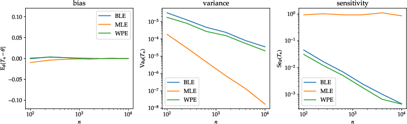
- Laplace location: choose the sample mean (BLE) over the sample median (MLE) when additive noise is present; the median’s sensitivity is constant in n, but the mean’s sensitivity scales as 2/n.
- Uniform scale: avoid the MLE (sample max; constant sensitivity), prefer BLE (2×mean; ~4/n sensitivity) or the paper’s WPE-inspired L-statistic.
- Linear regression: OLS is sensitivity-optimal in DWS models with centered errors; avoid estimators relying heavily on a few datapoints (e.g., stepwise selection via a single residual threshold).
- Variance estimation under Gaussian mean-uncertainty: the sample variance is asymptotically sensitivity-optimal.
- Tools/workflows: compute or empirically estimate Senθ(Tₙ), compare to the WCR bound; switch to BLE/WPE/L-statistics where appropriate; document both variance and sensitivity in model selection memos.
- Assumptions/dependencies: additive Gaussian-like perturbations; i.i.d. data; model satisfies differentiability in the Wasserstein sense (DWS) or sensitivity can be reliably estimated; unbiased or asymptotically unbiased estimators.
- Stability auditing and reporting alongside variance
- Use case: Add a “sensitivity” metric to model cards, validation reports, and governance documents to quantify how much estimator outputs change under small input noise.
- Sectors: software/ML platforms, regulated analytics (healthcare, finance), A/B testing infrastructure.
- Tools/workflows: compute Senθ(Tₙ) analytically where possible; otherwise, estimate ε-sensitivity via Monte Carlo with small ε and extrapolate to sensitivity; compare to theoretical WCR bound to assess near-optimality.
- Assumptions/dependencies: small-ε regime approximates operational perturbations; access to a plausible parametric model and the ability to simulate local noise around observed data.
- Privacy-preserving analytics under additive local noise
- Use case: When local differential privacy (LDP) or client-side randomization is implemented via calibrated additive noise, use sensitivity to anticipate utility loss and to pick estimators that minimize it.
- Sectors: privacy engineering (mobile telemetry, decentralized surveys), ad-tech.
- Tools/workflows: quantify MSE inflation ≈ noise_variance × Senθ(Tₙ); choose estimators with smaller sensitivity; set noise scales to meet utility/privacy targets.
- Assumptions/dependencies: additive mechanisms (e.g., Gaussian/Laplace) dominate the privacy design; unbiasedness or small bias; local noise is independent of data.
- Fast robustification via small-radius DRO approximations
- Use case: Use sensitivity as a first-order approximation to increase loss/risk under Wasserstein ambiguity sets of small radius, for quick robust optimization without solving full DRO programs.
- Sectors: finance (portfolio optimization), supply chain, pricing under demand uncertainty.
- Tools/workflows: robust risk ≈ nominal risk + ε × sqrt(Senθ(Tₙ)); use to screen policies or to size ambiguity sets; integrate into scenario analysis dashboards.
- Assumptions/dependencies: Wasserstein ambiguity sets are appropriate; small-radius regime; differentiability of objectives.
- 1D Wasserstein projection estimator (WPE) for robust parametric fitting
- Use case: Replace MLE with WPE when MLE is brittle under input noise, especially in 1D models where WPE is reducible to quantile computations.
- Sectors: economics (income distributions), operations (lead time modeling), reliability (lifetime data), actuarial science.
- Tools/workflows: compute WPE via quantile matching/monotone transport; use asymptotic sensitivity-efficiency to justify estimator choice; implement in R/Python using quantile transport.
- Assumptions/dependencies: parametric model well-specified; 1D outcome; computationally tractable W₂ projection.
- Sensitivity-aware A/B testing and telemetry analytics
- Use case: Prefer estimators that average across many observations (low sensitivity) rather than those driven by extreme values (high sensitivity), especially when client-side noise, jittering, or coarse sensors are present.
- Sectors: software experimentation, digital marketing, product analytics.
- Tools/workflows: report both standard errors and sensitivity; replace metrics based on maxima/medians with means or L-statistics when appropriate; validate with ε-sensitivity simulations.
- Assumptions/dependencies: perturbations resemble small additive noise; stable sampling scheme; unbiasedness is preserved or bias is negligible at the experiment’s scale.
- Day-to-day data summarization in noisy settings
- Use case: For personal health or home IoT dashboards, prefer averages (or tailored L-statistics) over maxima/medians when the device is noisy and outliers are not the primary concern.
- Sectors: consumer apps, personal analytics.
- Tools/workflows: settings toggles for “noise-stable summaries”; explain trade-offs between robustness (to outliers) and sensitivity (to small perturbations).
- Assumptions/dependencies: small, pervasive noise is the dominant issue; users understand the trade-off with outlier robustness.
Long-Term Applications
These depend on further research, scaling, or ecosystem development (statistical OT theory, algorithms, and tooling).
- Scalable WPE for high dimensions and semi-discrete OT
- Use case: Make WPE a general-purpose substitute or complement to MLE in multivariate models, with guarantees and efficient solvers.
- Sectors: machine learning, imaging, remote sensing, geospatial analytics.
- Tools/products/workflows: GPU-accelerated OT solvers; statistical guarantees for potentials’ higher-order derivatives; diagnostics for Laguerre cell ellipticity; libraries exposing WPE with gradients.
- Assumptions/dependencies: advances in semi-discrete OT theory and numerics; stable, scalable power diagram computations; verified DWS conditions.
- Sensitivity-optimal estimators for complex models via transport families
- Use case: Extend transport-family characterization to GLMs, time series, hierarchical/causal models, yielding exactly or asymptotically sensitivity-efficient estimators.
- Sectors: biostatistics, industrial forecasting, econometrics.
- Tools/products/workflows: symbolic/automatic derivation of Φθ, Λ(θ), J(θ); estimator synthesis modules returning L-statistics or projections tailored to χ(θ).
- Assumptions/dependencies: model-specific DWS verification; existence of unbiased or bias-corrected estimators; tractable computation of Λ(θ) and J(θ).
- AutoML and MLOps with sensitivity-aware model selection
- Use case: Incorporate sensitivity as a selection/regularization criterion alongside bias, variance, and calibration; penalize high Dirichlet energy of estimators.
- Sectors: ML platforms, forecasting services.
- Tools/products/workflows: add sensitivity penalties to loss functions; cross-validate with sensitivity-aware criteria; dashboards tracking sensitivity drift as data quality changes.
- Assumptions/dependencies: differentiable estimators or surrogates; reliable sensitivity estimation under distribution shift.
- Privacy and policy: standards for sensitivity-aware public statistics
- Use case: Statistical agencies that add noise to protect privacy calibrate both noise scales and estimators using sensitivity to maximize utility under mandated privacy budgets.
- Sectors: government statistics, health surveillance, education data.
- Tools/products/workflows: publication guidelines including WCR-based lower bounds; sensitivity scorecards for released statistics; estimator libraries approved for specific releases.
- Assumptions/dependencies: formal mapping between privacy mechanisms and additive noise models; acceptance of W₂-based local perturbation analyses in policy frameworks.
- End-to-end sensing system design co-optimizing hardware noise and estimator sensitivity
- Use case: Jointly design sensor specifications and analytics to meet end-to-end accuracy targets under budget and power constraints.
- Sectors: automotive, aerospace, smart grids, industrial automation.
- Tools/products/workflows: sensitivity enters system-level error budgets; estimator design tailored to sensor noise profiles; procurement specs include sensitivity thresholds.
- Assumptions/dependencies: additive noise dominates other error sources; component variances are stable over time and conditions.
- Robust risk management with Wasserstein ambiguity informed by sensitivity
- Use case: Size ambiguity sets dynamically using sensitivity to control worst-case risk without excessive conservatism; deploy in production risk engines.
- Sectors: finance, insurance, supply chain risk.
- Tools/products/workflows: sensitivity-calibrated DRO; monitoring that adjusts ε as data quality or market microstructure noise changes.
- Assumptions/dependencies: W₂ is the right geometry for uncertainty; small-ε expansions remain accurate in operational ranges.
- Fairness and interpretability via Wasserstein projections
- Use case: Project complex empirical distributions onto interpretable parametric families (e.g., monotone shifts, location-scale models) using WPE to improve communicability and enforce structural constraints.
- Sectors: regulated AI, HR tech, credit scoring.
- Tools/products/workflows: constrained WPE incorporating fairness constraints; audit tools comparing empirical vs projected distributions.
- Assumptions/dependencies: computationally tractable constrained OT; legal acceptance of Wasserstein-based projections as explanations.
- Educational and methodological infrastructure
- Use case: Incorporate sensitivity and WCR bounds into statistical curricula and software (e.g., R/Python packages) to normalize dual reporting of variance and sensitivity.
- Sectors: academia, scientific publishing.
- Tools/products/workflows: textbook modules; simulation notebooks demonstrating variance–sensitivity trade-offs; replication packages for example models (location, scale, regression, uniform).
- Assumptions/dependencies: community adoption; stable APIs for OT primitives.
Notes on feasibility across applications:
- The theory is sharpest for i.i.d. data, additive perturbations, and parametric models satisfying DWS; in heavy-tailed, dependent, or non-additive noise settings, empirical sensitivity estimation and robustness checks are recommended.
- WPE is straightforward in 1D and selected special cases; general high-dimensional deployment awaits advances in semi-discrete OT and solver stability.
- Many benefits accrue even without exact J(θ): Monte Carlo ε-sensitivity approximations often suffice for ranking estimators and informing design choices.
Glossary
- Ambiguity set: A set of probability distributions considered plausible alternatives to the empirical distribution in robust optimization. "ambiguity set taken to be Wasserstein balls of small radius"
- Asymptotic efficiency: The property of an estimator achieving the smallest possible asymptotic variance among a class of estimators. "asymptotic efficiency of maximum likelihood estimation"
- Best linear estimator (BLE): The estimator that is linear in the data and minimizes mean squared error (or variance) among linear unbiased estimators. "the best linear estimator (BLE) given by twice the sample mean"
- Breakdown point: The largest fraction of contamination an estimator can handle before it yields arbitrarily bad results. "its breakdown point is \sfrac{1}{2}"
- Continuity equation: A PDE describing mass-conserving flows of probability measures via a velocity field. "\partial_t\mu_t +\textnormal{div}(v_t\mu_t)=0"
- Cosensitivity matrix: A matrix-valued measure of sensitivity for vector-valued estimators, analogous to a covariance matrix. "cosensitivity matrix which is analogous to the covariance matrix."
- Cramér-Rao lower bound: A fundamental lower bound on the variance of unbiased estimators in terms of Fisher information. "Cram " er-Rao lower bound"
- Dirichlet energy: An integral of squared gradients that quantifies the “roughness” or sensitivity of a function. "the notion of the Dirichlet energy studied in probability theory, partial differential equations, and potential theory"
- Differentiability in quadratic mean (DQM): A smoothness condition on statistical models enabling classical asymptotic theory and Fisher information. "differentiability in quadratic mean (DQM)"
- Differentiability in the Wasserstein sense (DWS): A smoothness condition on statistical models based on optimal transport linearizations. "differentiability in Wasserstein sense (DWS)"
- Distributionally Robust Optimization (DRO): An optimization framework minimizing worst-case expected loss over an ambiguity set of distributions. "Distributionally Robust Optimization (DRO)."
- Empirical measure: The discrete probability measure placing mass 1/n on each observed data point. "the empirical measure of "
- Exponential family: A class of distributions whose densities have linear sufficient statistics and possess optimal variance properties. "exponential family"
- Fisher information matrix: The matrix capturing curvature of the log-likelihood; it bounds the variance of unbiased estimators. "Fisher information matrix"
- Fisher-Rao geometry: A Riemannian geometric structure on probability distributions induced by Fisher information. "the Fisher-Rao (equivalently, Hellinger) geometry"
- Geodesic: The shortest-path curve (with constant speed) between two points under a given metric. "constant-speed geodesic"
- Hellinger distance: A metric on measures defined via the L2 distance between square roots of densities. "squared Hellinger distance"
- Hellinger geometry: The geometric structure on measures induced by the Hellinger metric. "Hellinger geometry"
- Influence function: A tool from robust statistics measuring the effect of infinitesimal contamination on an estimator. "influence functions"
- Kullback-Leibler (KL) divergence: A measure of discrepancy between probability distributions based on relative entropy. "Kullback-Leibler (KL) divergence"
- Laguerre cells: The convex polytopes of a power diagram used to describe semi-discrete optimal transport partitions. "Laguerre cells in a random power diagram."
- Laplace distribution: A distribution with density proportional to exp(−|x−θ|), often leading to median-based estimators. "Laplace distribution with mean and variance 2"
- L-statistics: Estimators that are linear combinations of order statistics. "class of -statistics"
- Local Differential Privacy (LDP): A privacy model where each data point is randomized at source before aggregation. "Local Differential Privacy (LDP)."
- Log-Sobolev inequality: A functional inequality linking entropy and Dirichlet energy, used to control variances and concentrations. "log-Sobolev inequality"
- Maximum likelihood estimator (MLE): The parameter value maximizing the likelihood of observed data under a model. "maximum likelihood estimator (MLE)"
- Minimum-distance estimator: An estimator defined by minimizing a statistical distance between the model and empirical distributions. "minimum-distance estimator"
- Optimal potentials: Solutions to dual optimal transport problems whose derivatives induce transport maps and partitions. "optimal potentials"
- Optimal transport: The study of moving probability mass optimally with respect to a cost function, often quadratic. "optimal transport"
- Optimal transport map: The map pushing one distribution to another while minimizing transportation cost. "optimal transport map from to "
- Order statistics: The sorted sample values from smallest to largest. "order statistics of "
- Ordinary least squares (OLS): The linear regression estimator minimizing squared residuals. "ordinary least squares (OLS) estimator"
- Poincaré inequality: A functional inequality bounding variance by Dirichlet energy (or gradient norms). "Poincar " e inequality"
- Power diagram: A weighted generalization of Voronoi diagrams used in semi-discrete transport. "power diagram"
- Reaction equation: An ODE representing measure evolution by local reweighting rather than transport. "reaction equation"
- Riemannian manifold: A smooth space equipped with smoothly varying inner products on tangent spaces. "a Riemannian manifold is, strictly speaking, a pairing "
- Score function: The gradient (in parameter) of the log-likelihood; central to classical information geometry. "score function"
- Semi-discrete optimal transport: Optimal transport problems between a continuous distribution and a discrete one. "statistical semi-discrete optimal transport"
- Sensitivity: A measure of an estimator’s responsiveness to infinitesimal additive perturbations of the data. "we refer to this as the ``sensitivity'' of an estimator."
- Tangent space: The linear space of feasible infinitesimal directions at a point on a manifold or metric measure space. "tangent space denoted by $\Tan_x(M)$"
- Transport family: A model class whose transport linearization factors through specific feature gradients, enabling exact sensitivity efficiency. "transport family"
- Transport linearization: The first-order approximation of optimal transport maps with respect to parameters. "transport linearization function"
- Wasserstein balls: Sets of distributions within a fixed Wasserstein distance from a reference distribution. "Wasserstein balls of small radius"
- Wasserstein-Cramér-Rao bound: A lower bound on estimator sensitivity in terms of Wasserstein information. "Wasserstein-Cram " er-Rao bound"
- Wasserstein geometry: The Riemannian-like structure on probability measures induced by optimal transport costs. "Wasserstein geometry"
- Wasserstein information matrix: The analog of Fisher information defined via transport linearizations. "Wasserstein information matrix"
- Wasserstein metric: The optimal transport distance between probability measures, typically W2 with quadratic cost. "Wasserstein metric"
- Wasserstein projection estimator (WPE): An estimator projecting the empirical measure onto the model by minimizing Wasserstein distance. "Wasserstein projection estimator (WPE)"
Collections
Sign up for free to add this paper to one or more collections.