The Geometry of Grokking: Norm Minimization on the Zero-Loss Manifold
Abstract: Grokking is a puzzling phenomenon in neural networks where full generalization occurs only after a substantial delay following the complete memorization of the training data. Previous research has linked this delayed generalization to representation learning driven by weight decay, but the precise underlying dynamics remain elusive. In this paper, we argue that post-memorization learning can be understood through the lens of constrained optimization: gradient descent effectively minimizes the weight norm on the zero-loss manifold. We formally prove this in the limit of infinitesimally small learning rates and weight decay coefficients. To further dissect this regime, we introduce an approximation that decouples the learning dynamics of a subset of parameters from the rest of the network. Applying this framework, we derive a closed-form expression for the post-memorization dynamics of the first layer in a two-layer network. Experiments confirm that simulating the training process using our predicted gradients reproduces both the delayed generalization and representation learning characteristic of grokking.
Paper Prompts
Sign up for free to create and run prompts on this paper using GPT-5.
Top Community Prompts
Explain it Like I'm 14
Overview
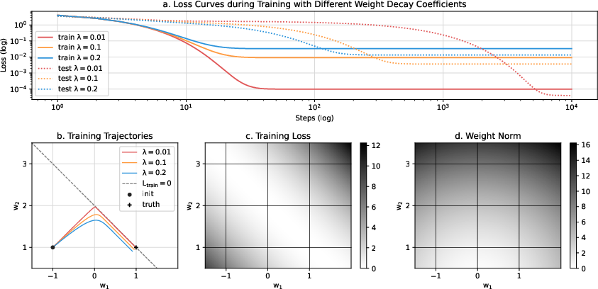
This paper tries to explain a strange thing that sometimes happens when training neural networks, called “grokking.” Grokking is when a model first memorizes the training examples perfectly, but only much later suddenly learns the real rule behind them and starts doing great on new, unseen examples. The authors show that once a model has memorized the training data, training behaves like a special kind of optimization: the model shrinks its weights as much as possible while keeping the training loss at zero. This shrinking, driven by “weight decay,” pushes the model toward simpler, cleaner internal representations that generalize.
Key Questions
The paper focuses on two main questions:
- What exactly does weight decay do after the model has memorized the training data?
- Can we study the learning of just one important part of the network (like the first layer that makes embeddings) without getting lost in the whole network’s complexity?
Methods and Approach (Explained Simply)
Think of training as walking downhill on a landscape of “loss,” where lower is better. Weight decay is like carrying a backpack with a rope that always tries to pull you toward the origin (smaller weights). Once the model reaches “zero loss” (it memorizes the training data), there’s a whole “zero-loss manifold” — a set of weight settings that all give perfect training results. Along this set, you can still move without increasing training loss.
The authors show that, near this zero-loss set, two things happen:
- The usual loss gradient (the main downhill direction) stops mattering along the set — it points perpendicular to the directions that keep loss zero. In plain terms: once the model memorizes, the loss no longer guides where to move next within the perfect-fit zone.
- Weight decay takes over and pulls the weights inward, making them as small as possible while staying on the perfect-fit set. This is called “norm minimization on the zero-loss manifold.”
To make the problem easier, the authors also “isolate” the learning of a subset of the network’s parameters (like the first layer) by assuming the rest of the network quickly adapts to whatever the first layer does. This is like saying the first layer is the “slow” part and the second layer is the “fast” part. Under this assumption, they turn the whole training problem into a simpler “cost function” that depends mostly on the first layer. That lets them write down an equation for how the first layer will move during training after memorization.
They test these ideas on a task called modular addition (adding numbers but wrapping around a fixed size, like a clock). Prior work found that the model learns circular patterns in its embeddings — placing symbols around circles — which makes the addition rule easy to compute and generalize.
Main Findings
Here are the main findings, expressed in everyday terms:
- After the model has perfectly memorized the training data, training behaves like trying to make the weights as small as possible while not messing up the perfect training performance. This shrinking is caused by weight decay.
- The usual “loss gradient” no longer nudges the model within the perfect-fit zone; instead, weight decay becomes the key driver. So the model slides along the zero-loss set toward smaller weights.
- You can reasonably isolate the learning of the first layer by assuming the second layer quickly adjusts to the best choice for whatever the first layer does. Under this assumption, the authors write down a formula for how the first layer changes after memorization.
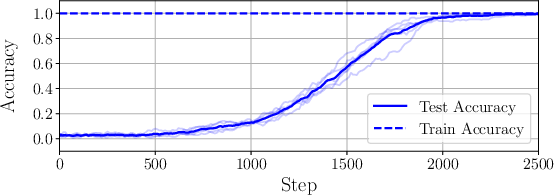
- When they simulate training using their predicted first-layer updates, they reproduce the grokking pattern: the model has zero training loss immediately but only later suddenly achieves high test accuracy. The embeddings form circles with neat geometric properties (equal sizes, orthogonal planes), matching what others have observed.
Why is this important? Making weights smaller tends to produce simpler internal “representations.” In this task, the simple representation is a circular layout that makes the addition rule easy and generalizable. So norm minimization explains how delayed generalization (grokking) happens: the model first memorizes, then slowly finds a simpler representation that works for new examples.
Implications and Impact
This work suggests a clear picture of what drives grokking: after memorizing, weight decay pushes the model to simplify itself while staying perfect on the training data, and that simplification can unlock generalization. Practically, this helps us:
- Understand training dynamics better, which can guide choosing training settings (like weight decay) to encourage good representations.
- Design methods that deliberately “nudge” models toward simpler, more generalizable internal structures.
- Build a bridge to studying specific parts of networks (like embeddings) in isolation, making it easier to analyze and improve them.
In short, if you want a model to truly learn the rule instead of just memorizing examples, it helps to let it first fit the data and then give it a gentle “shrink” toward simpler solutions. This paper explains why that process can lead to the sudden, surprising generalization we call grokking.
Knowledge Gaps
Knowledge gaps, limitations, and open questions
Below is a concise list of what remains missing, uncertain, or unexplored in the paper, framed to be concrete and actionable for future work.
- Finite-step, stochastic training: The analysis assumes continuous-time gradient flow and full-batch optimization; it does not quantify deviations under discrete updates, minibatch SGD noise, momentum, or adaptive optimizers (e.g., Adam/AdamW). Precise conditions and error bounds under realistic stochastic training remain open.
- Magnitude and scaling of weight decay: Results are proven in the limit , but practical training uses finite . How closely do trajectories follow the projected norm-minimization dynamics as a function of (and learning rate), and how does the grokking delay scale with ?
- Timescale separation and singular perturbation: The “fast loss minimization, slow norm minimization” intuition is not formalized (e.g., via geometric singular perturbation theory). Conditions guaranteeing a normally hyperbolic slow manifold and rigorously reducing dynamics to constrained norm minimization are not established.
- Loss landscape regularity: Key theorems assume smoothness and avoidance of singular points; real networks with ReLU are only piecewise smooth, and training can cross kinks. A formal extension handling nonsmooth activations (and measure-zero boundaries) and characterizing behavior near/between regions is missing.
- Behavior at/near singularities: The zero-loss set may have singular points (non-manifold structure). The dynamics and stability in their vicinity are not analyzed; robustness of the main claims to such degeneracies is unknown.
- Cross-entropy loss and logits at infinity: The work focuses on mean squared error. For cross-entropy/softmax, “zero loss” is typically achieved at infinite margin; the equivalent constrained manifold and the orthogonality/min-norm dynamics are not derived.
- Nonzero-loss regime: The theory assumes exact memorization. Many realistic settings never reach . How do the conclusions adapt to small-but-nonzero loss (e.g., constrained to low-loss tubes), and what is the impact on generalization dynamics?
- Isolated dynamics approximation (argmin over the complement): The assumption that instantly minimizes lacks conditions or error bounds. When (e.g., by layer-wise timescale separation, curvature, conditioning) is this a valid surrogate, and how large is the approximation error over time?
- Two-layer restriction: The isolated-dynamics derivation is limited to two-layer models. Extending closed-form or tractable approximations to deeper architectures (multi-layer, residual, attention) is an open challenge.
- Full-rank and invertibility assumptions: The derivation of uses or , requiring rank conditions that may fail (e.g., dead ReLUs, collinear features, limited data). A robust treatment (regularization, pseudoinverse properties, rank-deficiency dynamics) is not provided.
- Numerical stability and scalability: Computing and differentiating is and may be ill-conditioned at scale. Practical algorithms that approximate the derived dynamics efficiently (e.g., using iterative solvers or low-rank updates) are not explored.
- Lack of quantitative validation against real training: Experiments simulate the predicted dynamics rather than compare them to actual training trajectories. No metrics (e.g., gradient-field cosine similarity, path length, manifold distance over time) are reported to quantify the fidelity of the approximation.
- Limited task/domain breadth: Empirical validation is confined to modular addition with a single and architecture. The generality of the theory across different algorithmic tasks, real-world datasets that grok, and varied network sizes/hyperparameters remains untested.
- Dependence on data split and sample size: The effect of training fraction, dataset size, and noise on the onset and speed of grokking under the proposed dynamics is not characterized.
- Predictive timing of grokking: While toy examples suggest trends with , a general predictive theory for the time-to-generalization (as a function of , learning rate, width, rank of , and data fraction) is absent.
- Role of other regularizers and implicit biases: Only explicit weight decay is analyzed. Whether similar constrained-minimization dynamics emerge from other explicit regularizers (e.g., , spectral norm) or from the implicit bias of SGD without weight decay is not addressed.
- Projection mechanics onto the zero-loss manifold: The results qualitatively assert movement along available directions with loss keeping trajectories near . An explicit expression for the projected update (i.e., projection of onto the tangent space) and its error bounds are not provided.
- Global optimality on the manifold: The constrained norm-minimization problem on a nonconvex zero-loss manifold may have multiple minima. Conditions for uniqueness, convergence guarantees, and potential basin structures are not analyzed.
- Analytical link to circular embeddings: The experiments show Fourier feature behavior consistent with circles, but an analytical derivation from the constrained minimization (e.g., proving that DFT-aligned circular embeddings minimize under modular-addition constraints) is not provided.
- Effect of activation choice: Beyond noting ReLU, the dependence of the derived dynamics and emergent representations on activation function class (smooth vs piecewise linear, saturation) is unexplored.
- Layerwise or decoupled weight decay variants: Modern optimizers (e.g., AdamW) decouple weight decay from the loss gradient and may use per-layer coefficients. How these design choices alter the constrained-minimization picture is not analyzed.
- Non-orthogonal parameter partitions: The isolated-dynamics setup presumes an orthogonal split . Many architectures have intertwined parameterizations (e.g., norms tied by normalization layers). How to generalize the approximation to such settings is unclear.
- Batch normalization, residual connections, and attention: The theory does not address normalization dynamics, skip connections, or attention mechanisms, which can alter geometry and rank properties; applicability and modifications needed are open.
- Initialization dependence: The sensitivity of the post-memorization trajectory to initialization (e.g., which minimum-norm solution is selected) and whether the theory predicts or explains such selection is not studied.
- Robustness to label noise or data corruptions: How noise affects the zero-loss set geometry, the validity of the isolated-dynamics reduction, and the emergence of generalizable representations is unexplored.
- Reproducibility scope: While code for simulated dynamics is promised, hyperparameter sensitivity (e.g., step size in simulated ODE, numerical inversion tolerances) and seed control are not detailed, limiting rigorous reproducibility and benchmarking of the claims.
Practical Applications
Immediate Applications
Below are concrete, deployable use cases that leverage the paper’s findings on “norm minimization on the zero-loss manifold” and the isolated-dynamics approximation for subsets of parameters.
- Optimizer schedule: “memorize-then-minimize-norm”
- Sector: software/ML across domains (vision, tabular, small-data R&D)
- Use case: After training loss ≈ 0, switch to a phase where weight decay is emphasized and the loss is held near zero (e.g., by re-fitting the last layer exactly), to accelerate generalization via norm minimization along the zero-loss set.
- Tools/workflows: Two-phase training loop; increase weight decay or reduce LR; analytic last-layer refit every N steps.
- Assumptions/dependencies: Overparameterization; ability to reach (near) zero loss; MSE or squared-error-compatible last layer; small λ regime; stable refitting routine.
- Analytic last-layer training plugin (ridge/L2-closed-form)
- Sector: software, education, healthcare (clinical models with small data), finance (tabular forecasting), robotics (low-data adaptation)
- Use case: Alternate between solving W2 = (HᵀH + λI)⁻¹HᵀY and updating W1 with gradients, reducing compute and stabilizing training in small-data/overparameterized regimes.
- Tools/products: PyTorch/TF module that provides “analytic last layer” for MSE regression/classification via one-vs-all RLSC; incremental solvers for (HᵀH)⁻¹ updates.
- Assumptions/dependencies: Squared loss or RLSC surrogate for classification; full column rank or Tikhonov regularization; cost of matrix inverses scales with hidden size.
- Grokking diagnostics and alerts
- Sector: software/ML operations
- Use case: Monitor when training has entered the post-memorization regime (weight decay dominates). Trigger alerts or schedule changes when “distance to zero loss” is tiny but validation still lags.
- Tools: Metrics panel tracking training loss, parameter norm, ratio of weight-decay gradient norm to loss-gradient norm, last-layer refit consistency; simple proxy for gradient-tangent orthogonality (e.g., dominance of -θ vs. ∇L terms).
- Assumptions/dependencies: Access to gradients; proxies used because exact tangent-space computation is expensive.
- Targeted regularization for key components (e.g., embeddings)
- Sector: NLP/recommenders/algorithmic reasoning tasks
- Use case: Apply stronger weight decay or isolated-dynamics updates on embeddings (slow component) while keeping other layers adaptive (fast component) to induce beneficial representations.
- Tools/workflows: Layer-wise λ schedules; periodic analytic refit of upper layers; per-layer learning-rate decay.
- Assumptions/dependencies: The “slow–fast” decomposition holds; embeddings are the bottleneck for generalization in the task.
- Post-hoc fine-tuning for small datasets (generalization after memorization)
- Sector: healthcare (diagnostics on limited labeled data), finance (risk models; tabular), scientific ML
- Use case: If your model achieves near-0 training error rapidly, continue training under stronger weight decay (holding train loss near zero) to improve test performance without changing labels/models.
- Tools: Fine-tuning recipes; early memorization detection; norm-minimization phase controller.
- Assumptions/dependencies: Overparameterized models; low-noise labels; squared-error-compatible output layer or RLSC.
- Lightweight simulation/prototyping of training dynamics
- Sector: academia/research, AutoML prototyping
- Use case: Replace full training runs with isolated-dynamics simulation (first-layer gradient from the paper’s closed-form) to preview whether grokking-like representation learning will occur under a given setup.
- Tools: A simulator implementing the derived gradient for two-layer networks to rapidly test data splits, λ schedules, hidden sizes.
- Assumptions/dependencies: Two-layer approximation; MSE loss; overparameterization; smooth activation (ReLU is piecewise-smooth).
- Curriculum and data-split design for algorithmic tasks
- Sector: education, research (mechanistic interpretability)
- Use case: Choose training fractions and weight decay to reliably elicit delayed generalization on modular/arithmetic tasks for didactic demos and mechanistic studies.
- Tools: Notebooks that visualize Fourier features, norms, and orthogonality across training; reproducible labs.
- Assumptions/dependencies: Synthetic tasks or tasks with known latent structure; ability to reach zero loss.
- Safety/compliance checklist for overfitting remediation
- Sector: policy/compliance in regulated ML (health/finance)
- Use case: Operationalize “don’t stop at memorization” by adding a documented norm-minimization phase and logging of post-memorization dynamics before deployment.
- Tools: SOPs and audit artifacts showing post-memorization training, λ schedule, generalization improvements.
- Assumptions/dependencies: Regulators accept process evidence; tasks where zero (or near-zero) training loss is achievable.
- Online/embedded adaptation with analytic refits
- Sector: robotics/edge AI
- Use case: With few new samples, periodically re-fit the final layer exactly and update embeddings slowly, improving generalization without full retraining.
- Tools/workflows: On-device RLSC; low-rank updates to (HᵀH + λI)⁻¹; memory-efficient caches of activations.
- Assumptions/dependencies: Limited data regimes; modest hidden sizes for tractable inverses; numerical stability.
- Hyperparameter guidance for grokking regimes
- Sector: AutoML/ML engineering
- Use case: Constrain weight decay search ranges and schedules using the paper’s insight: smaller λ → better asymptotic norm but longer grokking delay; plan budgets accordingly.
- Tools: AutoML priors; adaptive λ annealing rules keyed to proximity to zero loss.
- Assumptions/dependencies: Detectability of near-zero loss; consistent overparameterization.
Long-Term Applications
These rely on extending the theory beyond current assumptions (e.g., cross-entropy loss, deeper networks) or on scaling/engineering advances.
- Optimizers that explicitly project onto the zero-loss manifold and minimize norm
- Sector: software/ML frameworks
- Use case: New training algorithms that alternate between projection to (near) zero loss and descent in parameter norm along the tangent space, accelerating grokking.
- Tools/products: “Manifold-projected optimizers” exposed as an optimizer class in PyTorch/TF.
- Assumptions/dependencies: Efficient approximations of projections; robust handling of singularities/nonsmooth activations.
- Generalization to cross-entropy and deep architectures
- Sector: mainstream ML (vision/NLP)
- Use case: Extend zero-loss manifold and norm-minimization dynamics to typical classification losses and multi-layer transformers/CNNs.
- Tools: Theoretical generalization; practical surrogates (e.g., temperature-scaled CE behaving like MSE near saturation).
- Assumptions/dependencies: New proofs/approximations; validated proxies for “near zero loss” under CE.
- Hardware/software acceleration for analytic refits
- Sector: systems/semiconductors/cloud ML
- Use case: Specialized kernels and incremental solvers for repeated ridge-regression updates inside training loops to make isolated-dynamics updates practical at scale.
- Tools/products: GPU/TPU kernels for batched (HᵀH + λI)⁻¹, Woodbury updates, mixed-precision stabilization.
- Assumptions/dependencies: Numerical stability; cost-model advantage over SGD-only loops.
- Federated/edge training with isolated components
- Sector: federated learning/IoT
- Use case: Clients perform local last-layer analytic fits; the server coordinates slower shared embedding updates, improving communication and convergence.
- Tools/workflows: Protocols for sharing sufficient statistics (HᵀH, HᵀY) instead of raw gradients.
- Assumptions/dependencies: Privacy-preserving aggregation of second-order stats; heterogeneity handling.
- Robustness and domain generalization via minimum-norm preference
- Sector: healthcare, finance, scientific ML
- Use case: Use constrained norm minimization along zero-loss sets to suppress spurious, high-norm memorizing solutions, improving OOD performance.
- Tools: Post-memorization “norm descent” phases; validators that probe spurious correlations before/after.
- Assumptions/dependencies: Spurious solutions correlate with larger norms; ability to maintain zero loss while moving to minimum-norm regions.
- Regulatory benchmarks and reporting for post-memorization dynamics
- Sector: policy/regulation
- Use case: Require developers to report training phases, weight-decay schedules, and post-memorization diagnostics to ensure models are not deployed in a pure memorization state.
- Tools: Standardized metrics (e.g., norm trajectories, “delay to generalization”).
- Assumptions/dependencies: Consensus on metrics; alignment with sector-specific risk frameworks.
- Automated “early grokking” detectors in training orchestration
- Sector: MLOps
- Use case: Pipeline controllers that detect entry into the zero-loss neighborhood and automatically switch optimizers/schedules to accelerate generalization or save compute.
- Tools: Controllers in Ray/Kubeflow; policies keyed to loss, norm, and gradient ratios.
- Assumptions/dependencies: Reliable detection signals; integration with schedulers.
- Representation-geometry shaping for reasoning/circuit discovery
- Sector: education, mechanistic interpretability, algorithmic reasoning
- Use case: Design regularizers that bias embeddings toward provably useful geometries (e.g., circles/torii) to elicit algorithmic circuits for arithmetic/group-structured tasks.
- Tools/products: Geometry-aware penalties; Fourier-feature monitoring libraries.
- Assumptions/dependencies: Task structure aligns with desired geometry; extension to multi-frequency/multi-plane structures.
- Post-training calibration through constrained norm descent
- Sector: general ML
- Use case: Post-training phase that holds predictions fixed on training data (zero-loss) while minimizing norm to improve generalization and calibration without retraining the full model.
- Tools: Constrained optimization wrappers; projected updates.
- Assumptions/dependencies: Reliable maintenance of zero training loss; stable projections in deep nets.
- Privacy and memorization control
- Sector: safety/privacy
- Use case: Reduce the risk of memorizing sensitive records by pushing away from high-norm, highly idiosyncratic solutions post-memorization.
- Tools: Privacy audits comparing memorization before/after norm-minimization phases; regularization policies.
- Assumptions/dependencies: Empirical link between norm-minimization and reduced record-level memorization; robust metrics for privacy leakage.
Notes on global assumptions and dependencies
- Core theory assumes: mean-squared error loss; overparameterization; ability to reach (near) zero training loss; vanishing weight decay regime; gradient-flow approximation; avoidance of singular points (measure-zero).
- Isolated-dynamics tooling assumes: two-layer networks (or linear last layer), solvable ridge regression, well-conditioned (HᵀH + λI), and differentiability of φ(θ₁).
- Practical considerations: numerical stability (regularize inverses), compute cost of matrix inversions, piecewise smoothness with ReLU, and the gap between continuous-time and discrete optimizers.
Glossary
- Available direction: A direction in parameter space along which one can move while staying on the zero-loss set; formally, a tangent direction that keeps loss at zero. "We say that is an available direction at if there exists a smooth trajectory such that , , and for all ."
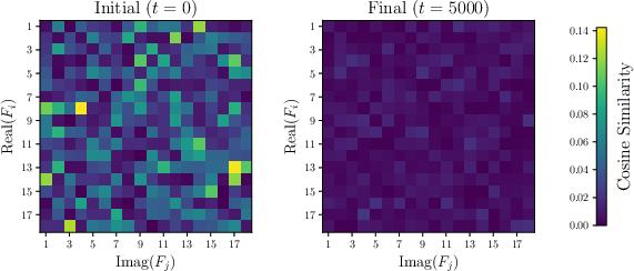
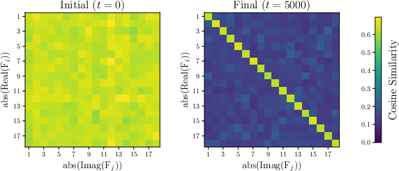
- Circular representations: Embeddings arranged on circles in latent space that enable symmetric algorithms (e.g., for modular addition). "circular representations emerge gradually during the post-memorization phase"
- Constrained optimization: Optimization of an objective subject to constraints; here, minimizing weight norm while remaining on the zero-loss manifold. "post-memorization learning can be understood through the lens of constrained optimization: gradient descent effectively minimizes the weight norm on the zero-loss manifold."
- Embedding matrix: The first-layer weight matrix that maps discrete tokens (e.g., one-hot vectors) to continuous embeddings. "we refer to the first layer weights as the embedding matrix ."
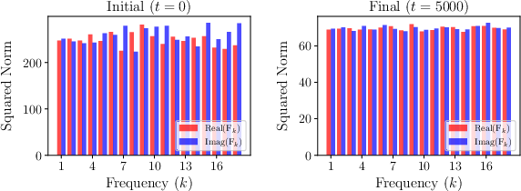
- Fourier features: Components obtained by decomposing embeddings via the discrete Fourier transform, revealing circular structures at different frequencies. "Fourier features norms equalize, suggesting the presence of equally-sized circles."
- Frobenius norm: Matrix norm equal to the square root of the sum of squared entries; used to measure weight magnitudes. "and denotes the Frobenius norm."
- Gradient flow: The continuous-time limit of gradient descent described by an ordinary differential equation. "we model the gradient descent trajectory as a continuous-time gradient flow:"
- Grokking: A phenomenon where generalization appears only after a long delay following perfect memorization. "Grokking is a puzzling phenomenon in neural networks where full generalization occurs only after a substantial delay following the complete memorization of the training data."
- Hadamard product: Element-wise multiplication of matrices or vectors. "and denotes the Hadamard product."
- Hessian matrix: The matrix of second derivatives of the loss; captures local curvature and determines tangent directions on the zero-loss set. "the tangent space is exactly the null space of the Hessian matrix"
- Inverse Function Theorem: A result ensuring local manifold structure of preimages when the Jacobian has full rank. "we directly restate the inverse function theorem below in a form that is slightly non-standard, but perfectly equivalent:"
- Jacobian matrix: Matrix of first derivatives of a vector-valued function; its rank characterizes singular points. "if the Jacobian matrix of at is not full rank"
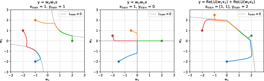
- Leaky ReLU activation: A ReLU variant with a small slope for negative inputs. "Right: a single-layer network with leaky ReLU activation groks simple addition."
- Lebesgue measure zero: Sets of zero measure under Lebesgue measure; events with probability zero in continuous settings. "a set of Lebesgue measure zero"
- Manifold: A space that locally resembles Euclidean space; here, the geometric structure of the zero-loss set. "The zero-loss subspace can more generally be thought of as a manifold"
- Moore–Penrose pseudo-inverse: A generalized inverse used to compute least-squares solutions, e.g., optimal linear layer weights. "also known as the Moore-Penrose pseudo-inverse of ."
- Normal space: The subspace orthogonal to the tangent space at a point on a manifold. "denote the normal space at a point ."
- Overparameterized: A regime where the model has more parameters than constraints, enabling exact memorization. "for the isolated learning dynamics of the first layer in the overparameterized zero-loss approximation:"
- Projection: Mapping a point to its closest point in a set (here, onto the zero-loss set). "be the projection of onto ."
- Ridge regression: Linear regression with L2 regularization; used to derive optimal second-layer weights. "equivalent to the classic problem of ridge regression"
- Singular points: Parameter values where the Jacobian loses rank, potentially breaking manifold structure. "We say that is a singular point"
- Tangent space: The set of directions at a point on a manifold along which one can move while remaining on the manifold. "the tangent space is exactly the null space of the Hessian matrix"
- Weight decay: L2 regularization on parameters that penalizes large weights and drives norm minimization. "We apply a weight decay term ... with a coefficient "
- Zero-loss manifold: The manifold of parameter values achieving zero training loss. "subject to remaining on the zero-loss manifold."
- Zero-loss set: The set of all parameter values with zero training loss. "Let denote the zero-loss set."
Collections
Sign up for free to add this paper to one or more collections.