Applications of AAA rational approximation
Abstract: The AAA algorithm for rational approximation is employed to illustrate applications of rational functions all across numerical analysis.
Paper Prompts
Sign up for free to create and run prompts on this paper using GPT-5.
Top Community Prompts
Explain it Like I'm 14
Overview
This paper is about a fast, reliable way to approximate complicated functions using rational functions (fractions of polynomials). The method is called the AAA algorithm. The authors show how AAA makes many tasks in numerical analysis easier, from quickly evaluating special functions to finding hidden features like poles and zeros. Their main goal is to explain what AAA can do, why it works, and where it helps in real problems.
What questions does the paper ask?
The paper explores simple, practical questions like:
- If we can easily build a rational function that closely matches a given function on a set of points, what new things can we do?
- How does this compare to traditional polynomial methods (like Taylor series)?
- How can we make the approximation both fast and accurate?
- Can we trust the results, and what should we watch out for (like fake poles)?
- How can we refine the approximation when we need the absolute best accuracy?
How does the AAA algorithm work? (Explained in everyday terms)
Think of AAA as a smart “copycat” system that learns a function by looking at its values and then builds a simple fraction that behaves the same way—almost everywhere you care about.
Here’s the idea in simple steps:
- You give AAA a bunch of points and the function values at those points (these are samples).
- AAA builds a rational function in a special format called the barycentric form. This format keeps the math stable and accurate, unlike the more fragile “p(z)/q(z)” format.
- AAA starts with a very simple approximation and improves it step by step. Each time, it looks at where its current guess is worst and adds a new “support point” there—like zooming in on the problem area.
- At each step, it solves a well-behaved linear algebra problem (using a tool called SVD, which finds the best fit) to adjust the weights of the support points. These weights tell the approximation how strongly to match the function at each point.
- It stops when the errors are tiny (usually near machine precision, around 13–15 digits for double precision).
Key words explained simply:
- Rational function: A fraction of two polynomials, like r(z) = p(z)/q(z).
- Poles and zeros: Special points where the function blows up (poles) or becomes exactly zero (zeros). These matter because they shape how the function behaves.
- Barycentric representation: A clever way to write rational functions that avoids numerical instability and loss of accuracy.
- Greedy algorithm: AAA keeps fixing the worst part first—like patching the biggest hole in a boat before the small leaks.
- SVD: A method that finds the best way to fit data with minimal error.
There are helpful variations:
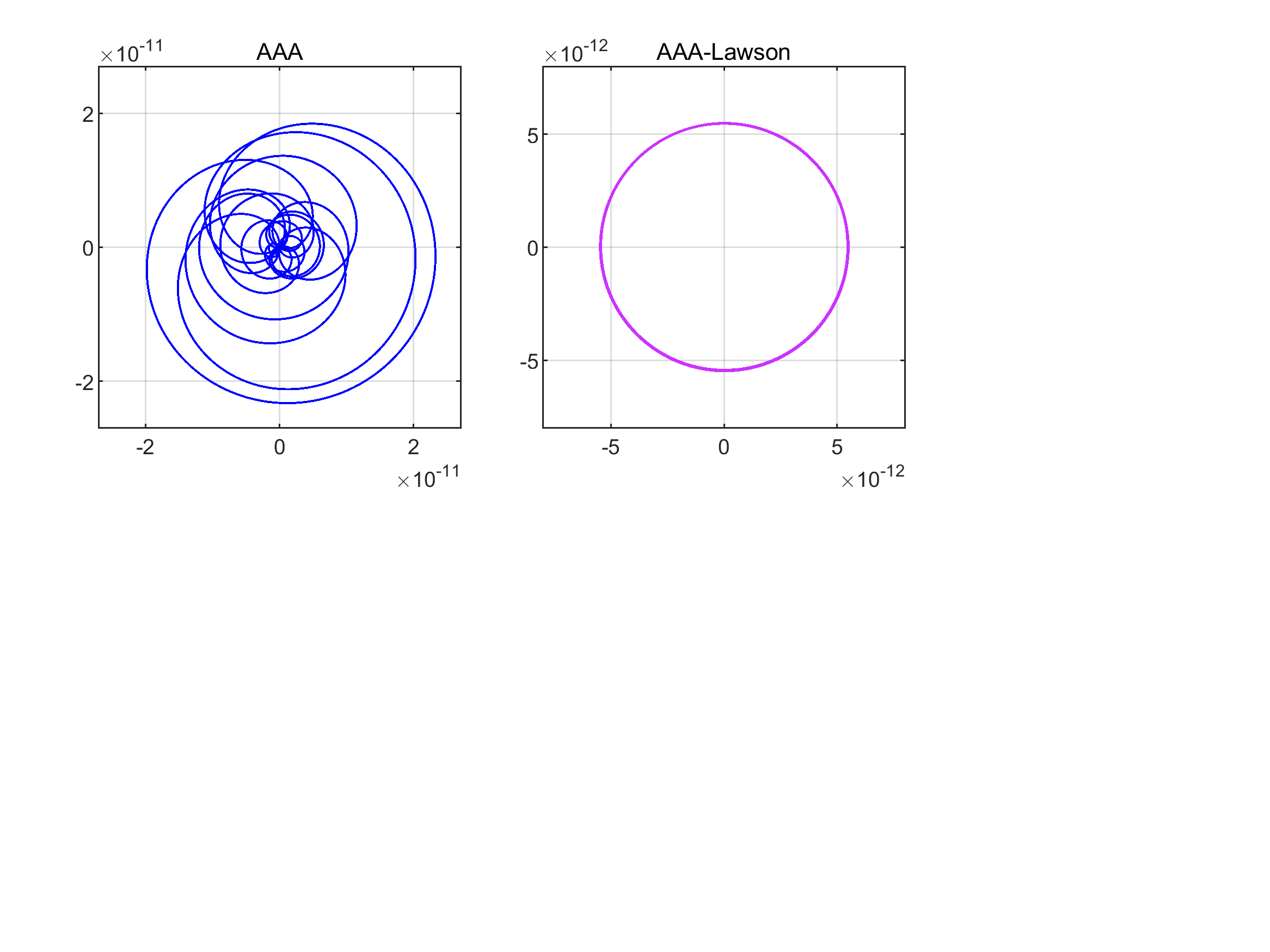
- AAA-Lawson: A refinement step that tweaks the approximation to be closer to the best possible of a given size.
- Continuum AAA: Works directly on continuous sets (like whole circles or intervals), not just discrete sample points.
- Symmetry tricks: If the data has complex conjugate symmetry, AAA can add points in conjugate pairs to keep the approximation real-symmetric.
What did the authors find, and why is it important?
Main takeaways:
- AAA is fast and simple: For moderate problem sizes (say, degree up to ~150), it usually runs in under a second on a laptop.
- It’s very accurate: Often reaches near machine precision (~13–15 digits).
- It works in many situations: On intervals, circles, scattered points, real or complex data, including functions with singularities.
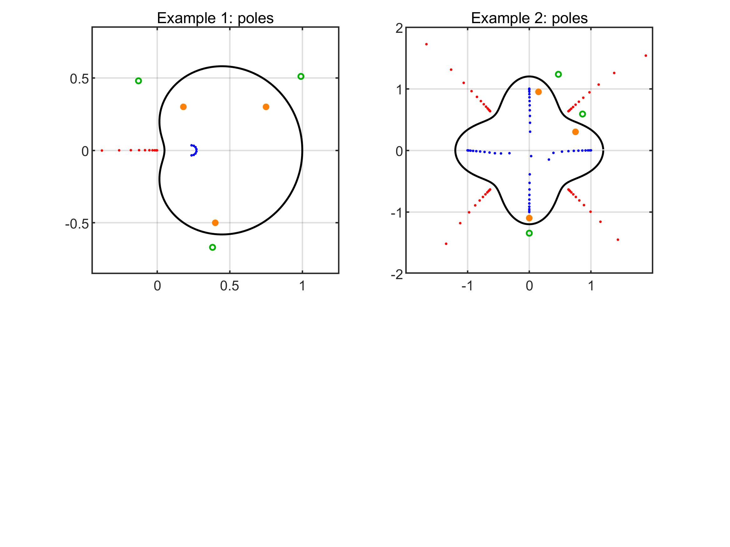
- It can “discover” features: AAA often pinpoints poles and zeros of the target function very accurately—even beyond the sampled region. This helps with understanding complex behavior and extrapolation.
- Rational beats polynomial in tough cases: When functions have sharp features or singularities, rational functions can approximate them much better and with far lower degrees. For example:
- If a function has branch points (sharp corners in its analytic structure), rational approximations converge “root-exponentially,” which is much faster than polynomials that only improve slowly.
- If the function is analytic except for poles, rational approximations can improve super fast, whereas polynomials improve only exponentially.
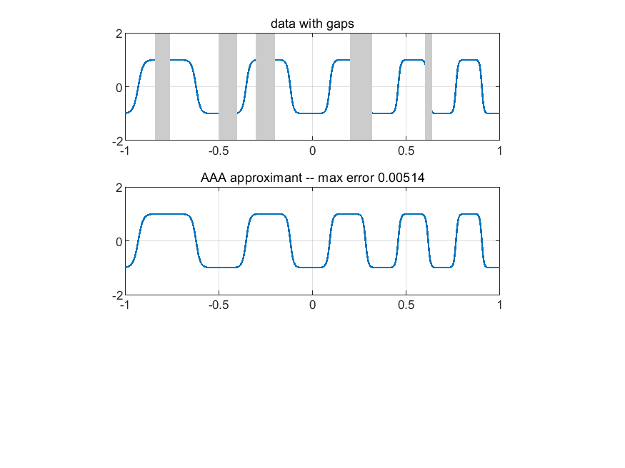
- It’s robust but not magic: AAA can sometimes produce tiny “spurious poles” (fake features caused by noise or limitations). There are cleanup tricks, and often these don’t harm accuracy away from the pole.
Examples from the paper (explained simply):
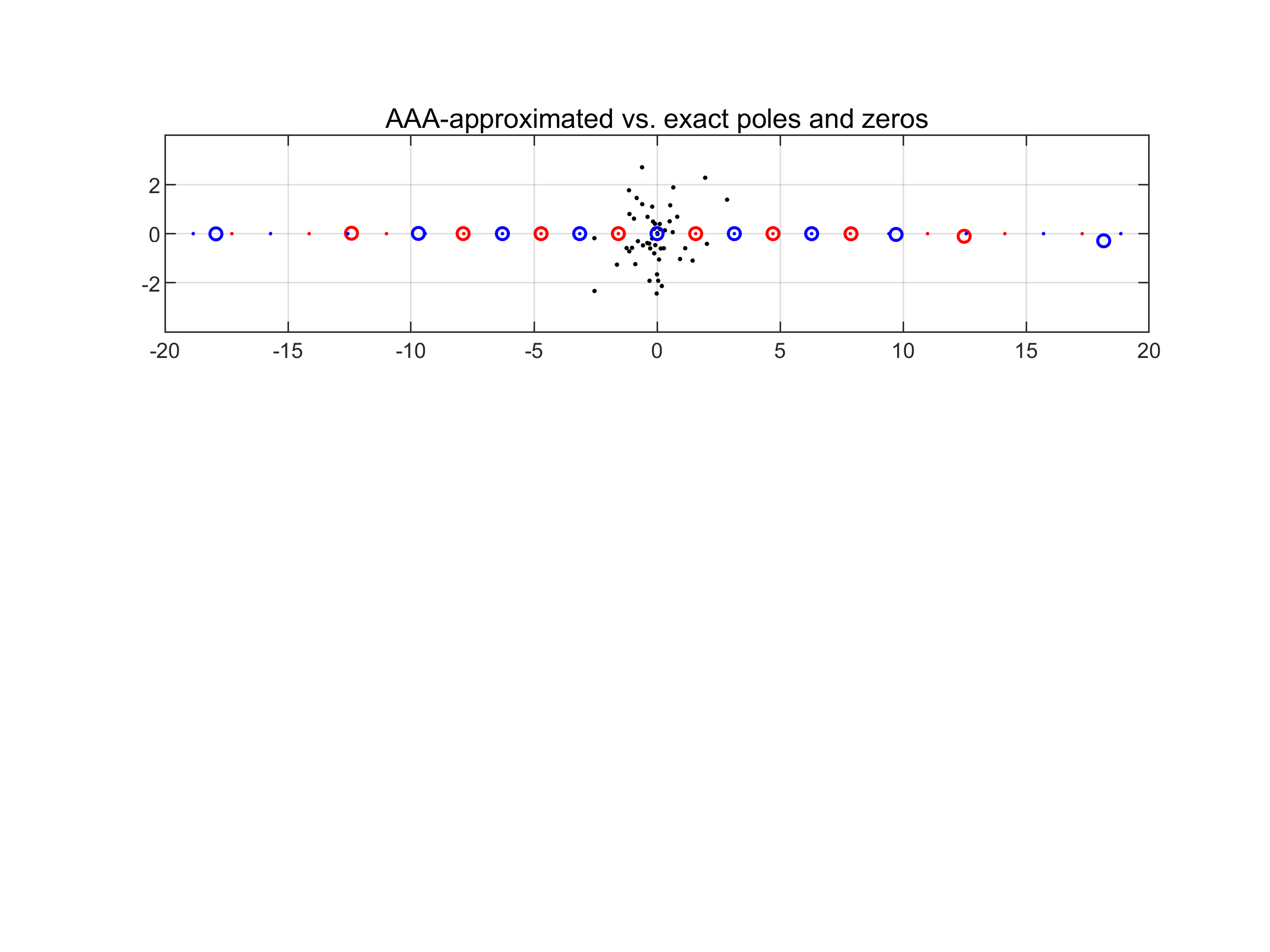
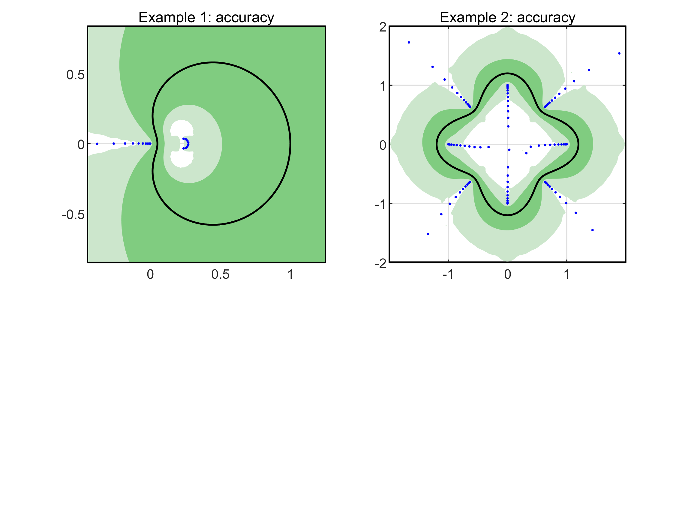
- Approximating tan(z) from scattered points: AAA got 11–14 correct digits at z=2 and accurately found nearby poles and zeros of tan(z), even those outside the sampled region.
- Approximating Γ(z) (the gamma function): AAA built very accurate rational copies on lines and circles, useful for fast complex evaluations.
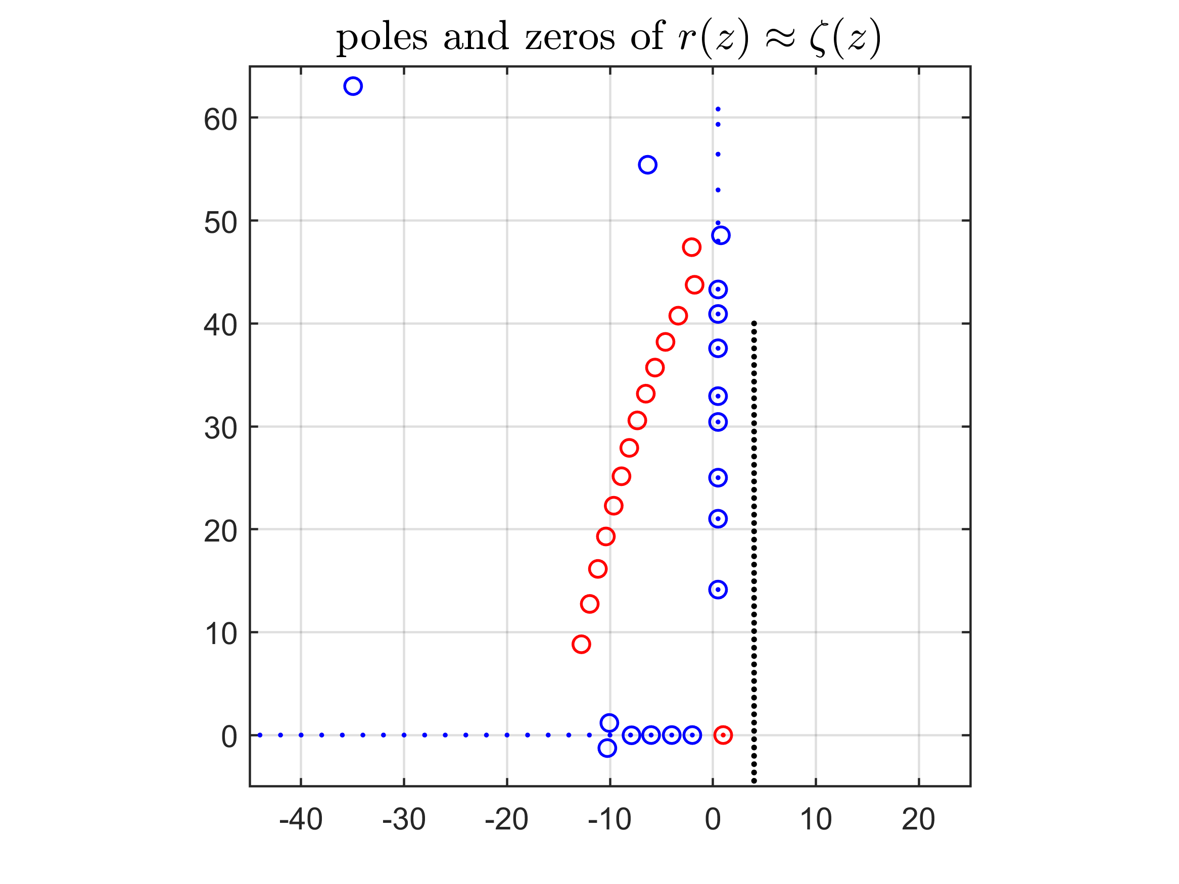
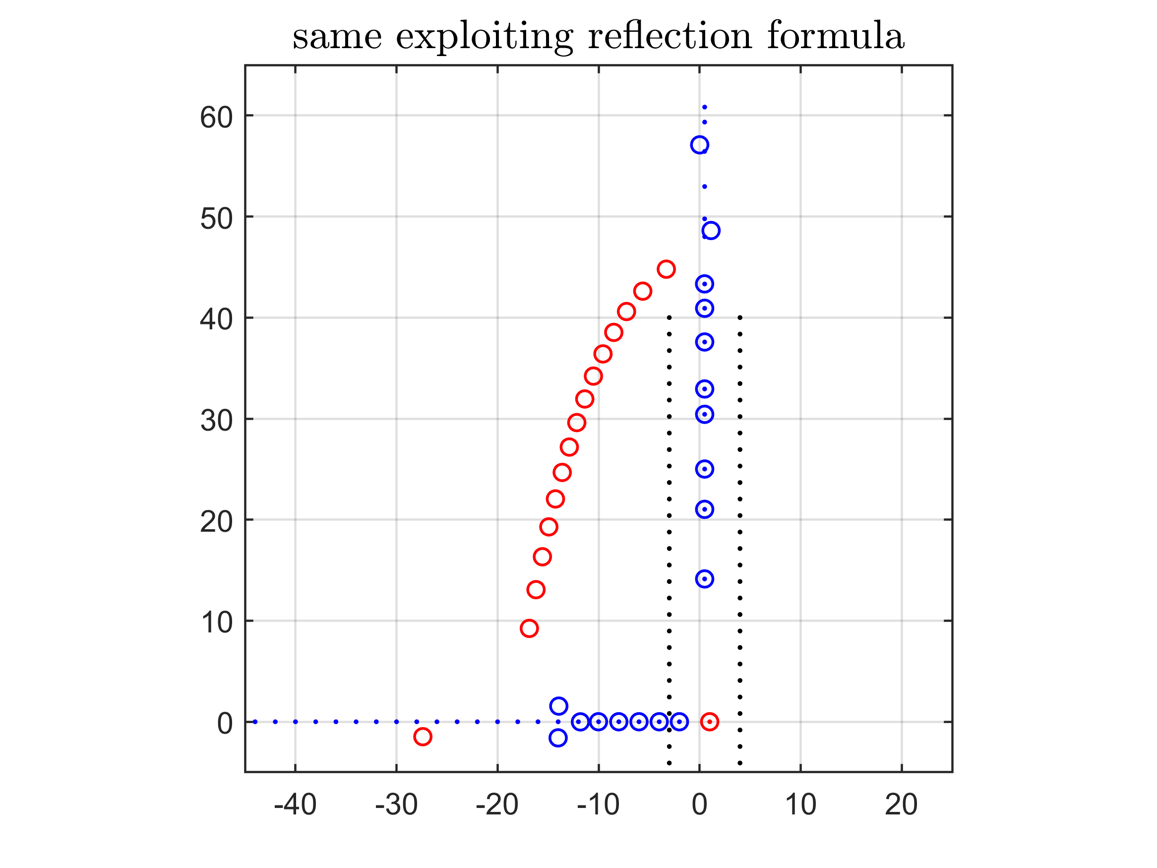
- Zeta function ζ(z): AAA used data on a vertical line to approximate ζ(z), correctly detecting its pole at z=1 and several zeros along the critical line.
Performance and practicality:
- Cost grows with the degree (roughly like n4), but for most applications they tried, that’s still fast.
- There are options to speed parts up or stabilize special cases (scaling columns, using more singular vectors, pairing conjugate points).
What does this mean for the future?
AAA opens a “new era” for rational approximation in numerical analysis:
- It turns previously hard tasks into almost plug-and-play tools.
- It’s available in common environments (MATLAB/Chebfun, Python/SciPy, Julia).
- It helps in building special function libraries, solving differential equations, designing filters, model reduction, and more.
- It enables better accuracy with smaller models, which saves time and memory.
- There are still open questions (like guarantees of “near-best” in all cases), and room to make the linear algebra even faster for very large problems.
In short: AAA makes rational functions practical for everyday scientific computing, often beating polynomials when functions have tricky behavior. It’s fast, accurate, and broadly useful—a powerful tool for modern math and engineering.
Knowledge Gaps
Knowledge gaps, limitations, and open questions
Below is a concise list of unresolved issues and open research directions explicitly or implicitly raised by the paper. Each item is formulated to be actionable for future work.
- Lack of theoretical guarantees of near-bestness: establish conditions under which AAA produces approximants within a provable factor of the degree‑n optimal rational approximation on a continuum domain E (not just accuracy on the discrete sample set Z).
- Discrete-to-continuum reliability: develop rigorous error bounds connecting convergence on a discrete set Z to uniform convergence on the intended continuum E, including explicit sampling density and distribution requirements to avoid “bad poles.”
- Control of pole locations: design and analyze constrained AAA schemes that prevent poles in forbidden regions (e.g., inside a real interval), with provable guarantees against spurious or interior poles.
- Spurious poles and Froissart doublets: provide robust, theoretically justified detection and cleanup procedures (including criteria for residue magnitude and pole–zero proximity), with proofs that cleanup preserves approximation quality.
- Sampling near singularities: automate and justify exponential clustering of sample points Z near branch points or other singularities to achieve root‑exponential convergence, including adaptive strategies that infer singularity locations during the run.
- Choice of tolerance and degree: develop principled, adaptive stopping criteria (tol, max degree n) informed by the analytic structure of f and the geometry of E, balancing accuracy, complexity, and risk of ill‑conditioning.
- Real symmetry enforcement: formalize and analyze symmetry-preserving AAA variants (e.g., conjugate‑pair support point insertion), including proofs of improved accuracy and stability, and generalizations to other symmetries (periodicity, reflection, problem‑specific invariances).
- Fast and scalable linear algebra: replace the O(n4) cost with provably stable and efficient algorithms (incremental/tall‑skinny SVD updates, randomized sketching) that retain accuracy; resolve stability issues with Gram/Cholesky approaches and quantify performance gains.
- Ill‑conditioning in the Loewner matrix: provide theoretical guidance for column scaling and for constructing weights from multiple right singular vectors (2025 adjustment), including criteria for when to apply these remedies and bounds on the resulting accuracy.
- Accuracy of computed poles, zeros, and residues: derive forward error bounds for poles/zeros/residues of the AAA approximant r in terms of Loewner matrix conditioning, sampling configuration, and proximity of poles to sample points.
- Residue computation methodology: analyze the new (2025) least‑squares residues method vs. the prior algebraic formula, with error bounds, stability proofs, and guidance on when each approach is superior.
- Continuum AAA maturation: turn continuum AAA into a standard tool with robust software and theory—establish convergence guarantees, pole control, sampling rules for boundary parameterizations, and complexity analyses on common domains.
- Partial fractions post‑processing: systematize the “acceptable pole” filtering and refitting in partial fractions form, including algorithms to select poles, quantify error changes, and guarantee numerical stability of the refit.
- AAA-Lawson reliability and speed: improve and analyze AAA‑Lawson (iteratively reweighted least squares) for robustness, especially near machine precision; develop convergence proofs, failure detection, and parameter‑tuning rules (e.g., number of Lawson steps).
- “Sign” and “damping” enhancements: provide a theoretical foundation and practical guidelines for the ‘sign’ and ‘damping’ features (as in zolo), including when they improve conditioning/accuracy and how to set parameters.
- Machine precision limitations: characterize when double precision prevents reaching true minimax behavior (e.g., ragged near‑circular error curves) and develop mixed‑precision/extended‑precision frameworks and triggers to switch precision reliably.
- Guidelines for sample set design: create actionable rules for choosing Z (size m, distribution on E, clustering near singularities, avoidance of near‑pole sample points), with quantifiable impact on accuracy and pole/zero fidelity.
- Robustness on real intervals: address AAA’s reduced reliability on real intervals (e.g., odd‑degree cases like |x|), by crafting interval‑specific variants or constraints that prevent interior poles while maintaining approximation quality.
- Extrapolation trustworthiness: quantify how far AAA approximations can be trusted outside the sampled region (analytic continuation), with bounds derived from potential theory/Hermite integrals tied to the chosen Z and the singularity landscape.
- Comparative benchmarking: perform systematic, application‑specific comparisons between AAA and alternative methods (Padé, Vector Fitting, IRKA, RKFIT, Thiele fractions), including success rates, accuracy, speed, and pole control, across diverse domains.
- Error metrics beyond ∞‑norm: study multi‑objective or weighted error criteria (e.g., RMS with constraints on max error) and extend AAA/AAA‑Lawson to optimize such metrics, with guarantees and practical algorithms.
- Parameter auto‑tuning: develop automated selection of AAA parameters (initial step, support point addition rules, termination, Lawson steps) driven by diagnostics (conditioning, error distribution, symmetry) to improve reliability and ease of use.
- Theoretical models for support point selection: analyze the greedy choice of support points (maximal error) and relate it to equioscillation/minimax theory, providing conditions under which this heuristic yields near‑optimal error curves.
- Integration with model reduction and control: clarify when AAA (and its variants) are competitive or complementary to established model reduction tools, providing theory and recipes for incorporating dynamics, stability, and structure preservation.
- Documentation and standardization across implementations: reconcile differences among MATLAB, Julia, Python implementations (e.g., symmetry, cleanup, residue computation), and publish a reference specification with test suites and reproducibility guidelines.
Practical Applications
Immediate Applications
Below is a curated set of practical applications that can be deployed now using the AAA algorithm and its available implementations. Each item notes sectors, likely tools/workflows, and key assumptions or dependencies that affect feasibility.
- Rational surrogate modeling from scattered samples
- Sectors: software engineering, scientific computing, applied mathematics
- Tools/workflows: Chebfun’s
aaa.m, SciPy/Python implementations, Julia packages; wrap function evaluations into a compact rational approximant; evaluate at new points with near machine precision - Assumptions/dependencies: The target function is meromorphic or well-approximable by rational functions; sample points cover regions of interest without pathological conditioning; set tolerances appropriately (e.g., loosen near singularities)
- On-the-fly analytic continuation and extrapolation near the data domain
- Sectors: physics, materials science, signal processing
- Tools/workflows: Fit AAA from data on an interval, circle, or scattered points; evaluate outside the sampling set to estimate values (e.g., gamma/zeta functions, transfer functions)
- Assumptions/dependencies: No “bad poles” in the evaluation region; use a posteriori pole/zero inspection; acceptable deviation due to extrapolation errors
- Pole–zero–residue extraction for black-box functions
- Sectors: RF/microwave engineering, control systems, power electronics, acoustics
- Tools/workflows: Compute poles/zeros via generalized eigenvalue problem on AAA barycentric form; validate stability margins, resonance locations, and network synthesis
- Assumptions/dependencies: Meromorphic behavior near the domain; sufficient sampling density; check for spurious poles/Froissart doublets and filter or refit via partial fractions least-squares
- Compact storage and transmission of measured or simulated curves
- Sectors: metrology, materials, energy, manufacturing QA
- Tools/workflows: Replace large tables with a low-degree barycentric rational model; ship coefficients instead of dense data
- Assumptions/dependencies: Data quality (noise may induce spurious poles); consider cleanup strategies; maintain metadata about approximation domain/tolerance
- Fast extension of special-function capabilities in environments lacking complex support
- Sectors: software libraries, education
- Tools/workflows: Create rational approximants for functions like Γ(z) or ζ(z) on specified domains; embed approximants in teaching tools or domain-specific apps
- Assumptions/dependencies: Reliability near machine precision; careful domain selection; ensure reflection formulas or known singularities are respected
- Rapid resonance identification and spectrum analysis
- Sectors: NDE (non-destructive evaluation), spectroscopy, structural dynamics
- Tools/workflows: Fit measured response curves to AAA, extract poles and residues; infer modal characteristics and damping
- Assumptions/dependencies: Adequate SNR; sample near resonances; validate residues via least-squares fit to mitigate numerical sensitivity
- System identification and compact transfer-function modeling
- Sectors: control engineering, robotics, automotive, aerospace
- Tools/workflows: Integrate AAA as an alternative/complement to Vector Fitting (VF), IRKA, RKFIT; enforce real symmetry by pairing conjugate support points; export models as partial fractions or state-space
- Assumptions/dependencies: Real-symmetry modifications; sampling strategies aligned with frequency content; handle ill-conditioning via column scaling or multi-vector weight constructions
- Robust evaluation near branch points and singular boundaries
- Sectors: computational physics, electromagnetics, computational fluid dynamics
- Tools/workflows: Use rational fitting for root-exponential convergence near branch points where polynomial methods fail; cluster sampling near singularities; relax tolerances for high-degree fits
- Assumptions/dependencies: Proper sample clustering near singularities; computational budgets for higher degrees (n ~ O(100–300) can be needed); monitor pole locations
- Simulation speed-ups via “fit once, evaluate many” surrogate loops
- Sectors: HPC, digital twin development, parametric studies
- Tools/workflows: Build AAA surrogates of expensive subroutines; cache and reuse; incorporate pole/zero validation for stability
- Assumptions/dependencies: Surrogate validity across required parameter ranges; automatic re-fitting when parameter drifts invalidate the model
- RF/microwave S-parameter compression and modeling
- Sectors: telecommunications, semiconductors, antenna design
- Tools/workflows: Use AAA (already in MATLAB RF Toolbox) to fit measured S-parameters; ensure real symmetry; export models for time-domain simulations
- Assumptions/dependencies: Enforce conjugate support points; verify passivity/causality separately (AAA fits the data but does not enforce those constraints by itself)
- High-accuracy pole/zero mapping for research in analytic number theory and complex analysis
- Sectors: academia (mathematics, theoretical physics)
- Tools/workflows: From line or circle samples of ζ(z) or other complex functions, map poles/zeros and explore behavior on critical lines; compare against known values
- Assumptions/dependencies: Accurate sampling strategies; potential use of reflection formulas; track approximation error growth away from data domain
- Teaching and prototyping tool for rational approximation and numerical analysis
- Sectors: education (undergraduate/graduate)
- Tools/workflows: Classroom demos using Chebfun/Julia/Python AAA implementations; illustrate barycentric forms, pole/zero computation, and error curves; extend with AAA-Lawson for minimax insights
- Assumptions/dependencies: Familiarity with numerical linear algebra; manage near-machine-precision effects (jagged error curves)
Long-Term Applications
The following opportunities require further research, scaling, or development (algorithmic, software, or theoretical) before wide deployment.
- Library-grade minimax rational approximations via AAA-Lawson
- Sectors: software libraries, scientific computing
- Tools/workflows: Use AAA as an initialization, then AAA-Lawson (iteratively reweighted least squares) for near-minimax; produce lower-degree/high-accuracy special-function libraries
- Assumptions/dependencies: AAA-Lawson stability near machine precision; “sign” and “damping” enhancements; robust stopping criteria; careful error certification
- Continuum AAA for boundary-based approximation and analytic continuation
- Sectors: computational geometry, PDE boundary value problems, complex analysis
- Tools/workflows: Fit on curves/regions (intervals, disks, circles, parameterized boundaries) without discrete sampling; integrate with boundary integral solvers
- Assumptions/dependencies: Mature tooling; parameterization quality; theoretical guarantees linking continuum fits to near-best rational approximants
- Rational spectral and boundary methods for PDEs/ODEs
- Sectors: engineering simulation, climate modeling, acoustics/electromagnetics
- Tools/workflows: Embed AAA-driven rational bases to treat corner singularities/inlets and improve convergence compared to polynomials; automate pole placement via fitting
- Assumptions/dependencies: Stable differentiation/integration operators in barycentric/partial fractions forms; spurious-pole mitigation; error estimation on complex domains
- Scalable AAA for large datasets via improved linear algebra
- Sectors: big data, ML, scientific HPC
- Tools/workflows: Develop stable O(n3) or randomized/sketched algorithms for the tall-skinny SVD/Loewner matrix; incremental Cholesky/QR updates with robust conditioning
- Assumptions/dependencies: Numerical stability of sketching/updates; consistent error control; careful treatment of Gram matrix conditioning
- Standards for rational surrogates in data repositories and policy guidance
- Sectors: public research agencies, standards bodies, open data policy
- Tools/workflows: Publish datasets with certified rational surrogates, domains of validity, and error/tolerance metadata; encourage reproducibility and efficient downstream use
- Assumptions/dependencies: Community consensus on formats and certification; tooling for validation and compliance; clear guidelines for singularity handling
- Fast pricing and risk analytics in quantitative finance using rational surrogates
- Sectors: finance
- Tools/workflows: Approximate characteristic functions or integrands with rational forms; exploit root-exponential convergence near branch cuts for speed; integrate in calibration loops
- Assumptions/dependencies: Domain-specific validation; robust extrapolation controls; sensitivity to market data noise
- Model-based diagnostics and control using pole-aware surrogates
- Sectors: robotics, autonomous systems, industrial control
- Tools/workflows: Online AAA fits to identify dynamics, then pole/zero monitoring for health checks; adaptive controllers with rational models
- Assumptions/dependencies: Real-time constraints; stability guarantees; passivity/causality enforcement layers atop AAA approximations
- Passivity/causality constrained AAA fits for EM and RF design
- Sectors: telecommunications, radar, IC design
- Tools/workflows: Combine AAA with constraint-enforcing post-processing (e.g., convex optimization) to guarantee physical realizability of fitted models
- Assumptions/dependencies: Efficient constrained fitting algorithms; robust error control; certification routines
- Automated pole cleanup and certification pipelines
- Sectors: cross-domain numerical modeling
- Tools/workflows: Standardized workflows that detect Froissart doublets/spurious poles, refit in partial fractions, and certify domain-safe pole locations; integrate in CI/CD for modeling assets
- Assumptions/dependencies: Reliable detection thresholds; reproducible refitting strategies; error certification on intended domains
- Multi-function/vector/matrix-valued AAA beyond scalar approximations
- Sectors: MIMO systems, networked control, multivariate signal processing
- Tools/workflows: Extend AAA to handle vector/matrix-valued responses, coupled poles/zeros, and multi-input/multi-output identification
- Assumptions/dependencies: Generalizations of barycentric representations; scalable pole/zero computations for block structures; stability and conditioning analyses
- Rational compression and analytics for scientific imaging and inverse problems
- Sectors: healthcare imaging, geophysics
- Tools/workflows: Employ AAA to compress forward models and kernels; accelerate iterative inversions via surrogate evaluations; use pole-zero analysis to understand artifacts
- Assumptions/dependencies: Validation against clinical/field datasets; domain-aware sampling; rigorous error bounds for reconstructions
- Education-to-industry transfer via robust open-source AAA ecosystems
- Sectors: education, software engineering
- Tools/workflows: Mature Julia/Python/Matlab AAA packages with documented best practices (real symmetry, Lawson steps, continuum AAA); tutorial curricula; integration examples across sectors
- Assumptions/dependencies: Community maintenance; cross-language consistency; example-rich documentation; pathways to certification for industrial adoption
These applications leverage the core innovations of AAA: a robust barycentric representation, a greedy descent strategy using Loewner matrices and SVD, optional symmetry and cleanup enhancements, and straightforward pole/zero computation. Feasibility hinges on thoughtful sampling, error tolerance selection, domain-appropriate checks for spurious poles, and—where needed—post-processing (e.g., AAA-Lawson, passivity/causality enforcement, partial-fractions refitting).
Glossary
- AAA algorithm: A greedy barycentric method for constructing rational approximations from sampled data. "Such an algorithm, the AAA algorithm, was introduced in 2018 \ccite{aaa}."
- AAA-Lawson algorithm: An extension of AAA that applies iteratively reweighted least squares (Lawson) steps to approach minimax (best L-infinity) rational approximations. "the extension of AAA known as the AAA-Lawson algorithm \ccite{aaaL}"
- Backward stability: A numerical property meaning the computed result is the exact solution for slightly perturbed input data. "one can say that they are backward stable in the usual sense of numerical linear algebra,"
- Barycentric representation: A numerically stable form expressing a rational function as a ratio of weighted sums over support points. "it employs a barycentric representation of a rational function rather than the exponentially unstable quotient representation ."
- Barycentric weights: The coefficients associated with support points in the barycentric formula. "The numbers are {\em barycentric weights},"
- Branch points: Points where a function is multi-valued or has non-isolated singularities, often causing algebraic convergence issues. "If has one or more branch points, then both polynomial and rational approximations converge"
- Chebfun: A software system (primarily MATLAB) for numerical computation with functions via piecewise polynomial/rational representations. "Many of these reliable methods are brought together in the Chebfun software system \ccite{chebfun}."
- Chebyshev polynomials: Orthogonal polynomials on [-1,1] widely used for stable approximation and interpolation. "often based on Chebyshev polynomials, Chebyshev points and Chebyshev interpolants \ccite{atap}."
- Cholesky factorisations: Decompositions of positive definite matrices used in linear algebra and fast updates. "(based on updating Cholesky factorisations)"
- Column scaling: Preconditioning technique that rescales matrix columns to improve conditioning and numerical stability. "Another is to apply column scaling to the matrix when it is highly ill-conditioned."
- Continuum AAA algorithm: A version of AAA that operates directly on continuous domains (e.g., curves) rather than discrete sample sets. "In the continuum AAA algorithm mentioned above \ccite{continuum}, poles are calculated at every step of the iteration."
- Dirichlet series: A series of the form used to define functions like the Riemann zeta function. "The function is defined by the Dirichlet series"
- Equioscillation: The alternation of equal-magnitude errors at optimally chosen points, characterizing minimax approximations. "a minimax approximation can be obtained with the Remez algorithm based on equioscillation,"
- Froissart doublets: Near-cancelling pole-zero pairs that often arise spuriously due to noise or numerical effects. "one also speaks of ``Froissart doublets’’ since these are poles that are paired with zeros"
- Generalised eigenvalue problem: An eigenproblem of the form used here to extract poles and zeros of rational functions. "their zeros can be found by solving the generalised eigenvalue problem"
- Gram matrix: A matrix of inner products whose factorization can be used in fast updates, though with stability caveats. "it is based on the Cholesky factorisation of the Gram matrix, which has stability issues associated with squaring the condition number."
- Greedy descent algorithm: An iterative method that makes locally optimal choices to reduce error rather than enforcing global optimality. "it is a greedy descent algorithm rather than aiming to enforce optimality conditions"
- Hermite integrals: Integral representations connected to approximation theory and used to analyze pole/zero localization. "most experts would connect the matter with Hermite integrals and potential theory,"
- IRKA: The Iterative Rational Krylov Algorithm for model reduction and rational approximation. "\ccite{irka} (``IRKA'')"
- Loewner matrix: A matrix with entries central to linearized rational approximation formulations. "known as a {\em Loewner matrix\/} \ccite{abg}."
- Meromorphic function: A function that is analytic except at isolated poles. "(A meromorphic function is one that is analytic apart from poles.)"
- Minimax approximation: Best uniform (infinity-norm) approximation minimizing the maximum absolute error over a set. "rational minimax (best -norm) approximations"
- Partial fractions form: Representation of a rational function as a sum of simple rational terms with distinct poles. "Both of these expressions are in partial fractions form,"
- Potential theory: A mathematical framework (harmonic/potential functions) underpinning asymptotic convergence results in approximation. "by arguments of potential theory to be outlined in section"
- QZ algorithm: The generalized Schur decomposition method for solving generalized eigenvalue problems. "Computing these eigenvalues using the standard QZ algorithm~\ccite{molerstewart} requires operations,"
- Randomised sketching: Techniques using random projections to reduce problem dimension and accelerate linear algebra. "(based on randomised sketching)."
- Reflection formula: A functional identity relating values of a function at and $1-z$ (e.g., for the Riemann zeta function). "where is evaluated by the reflection formula"
- Removable singularity: A point at which a function’s expression is singular but the function can be defined to be analytic. "Thus is a removable singularity of (\ref{aaa-baryrep}),"
- Residues: Coefficients of the principal part of a function at its poles, indicating pole strength. "the poles, residues and zeros of the approximation ."
- Remez algorithm: An algorithm to compute minimax (best uniform) polynomial or rational approximations. "a minimax approximation can be obtained with the Remez algorithm based on equioscillation,"
- Root-exponential convergence: Error decay of the form typical for rational approximation near branch singularities. "converge root-exponentially, i.e., at a rate "
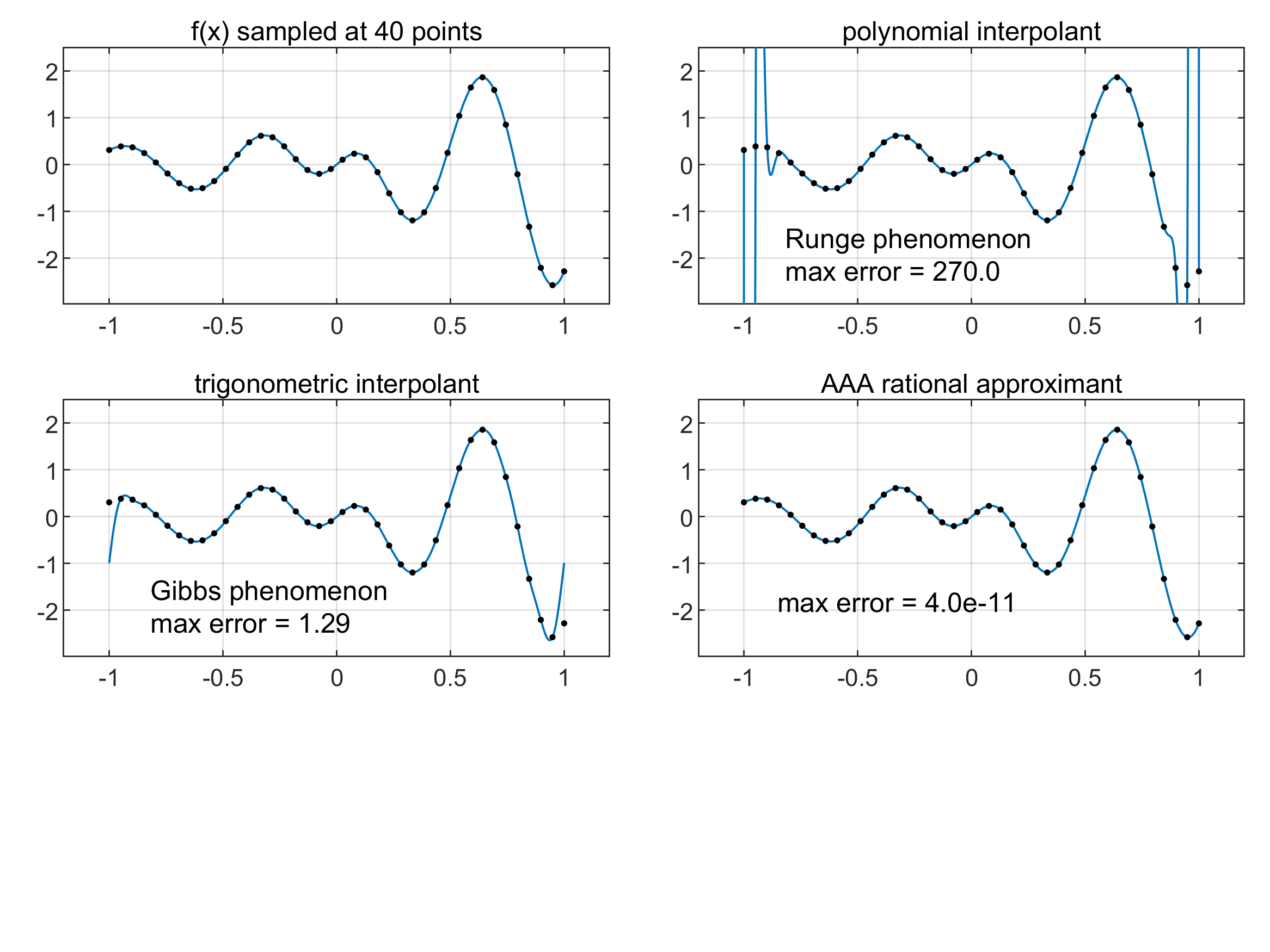
- Runge phenomenon: Instability/oscillation of polynomial interpolation at equispaced points on an interval. "the Runge phenomenon \ccite{atap}: interpolation of all the data does not ensure that anything useful has been achieved."
- Singular value decomposition (SVD): Matrix factorization used to compute barycentric weights in AAA. "computing the singular value decomposition (SVD) of "
- Support points (nodes): Selected sample points where the rational approximant interpolates the data in barycentric form. "The numbers , which are distinct entries of , are {\em support points} or {\em nodes}."
- Thiele continued fractions: A continued-fraction representation enabling greedy rational interpolation. "namely Thiele continued fractions \ccite{salazar,driscollzhou,driscolljuliacon}."
- Vandermonde with Arnoldi orthogonalisation: A stable procedure to build polynomial bases for fitting/interpolation. "(A well-conditioned basis for the polynomial can be constructed by Vandermonde with Arnoldi orthogonalisation~\ccite{VA}.)"
- Vector fitting: A practical algorithm for rational approximation by fitting frequency-domain data. "\ccite{vf} (``Vector fitting'')"
- Winding number: The number of times a curve wraps around the origin, used to assess near-optimality of error curves. "the error curve is approximately a circle of winding number 21 \ccite{nearcirc}."
Collections
Sign up for free to add this paper to one or more collections.