Generalization of Gibbs and Langevin Monte Carlo Algorithms in the Interpolation Regime
Abstract: The paper provides data-dependent bounds on the test error of the Gibbs algorithm in the overparameterized interpolation regime, where low training errors are also obtained for impossible data, such as random labels in classification. The bounds are stable under approximation with Langevin Monte Carlo algorithms. Experiments on the MNIST and CIFAR-10 datasets verify that the bounds yield nontrivial predictions on true labeled data and correctly upper bound the test error for random labels. Our method indicates that generalization in the low-temperature, interpolation regime is already signaled by small training errors in the more classical high temperature regime.

Paper Prompts
Sign up for free to create and run prompts on this paper using GPT-5.
Top Community Prompts
Explain it Like I'm 14
Overview
This paper studies when and why machine learning models that can perfectly fit their training data (even nonsense data) still make good predictions on new, unseen data. The authors focus on a theoretical learning rule called the Gibbs algorithm and on practical samplers known as Langevin Monte Carlo (LMC). They build new, data-dependent formulas (called bounds) that predict how well such models will do on test data, even in the tricky “interpolation” setting where training error is near zero.
What questions does the paper ask?
- Can we predict the test error of models that can memorize the training set (including random labels), using only the training data?
- Can we make such predictions for the Gibbs algorithm at any “temperature” (a knob that controls how much the algorithm prefers low training error)?
- If we can’t sample exactly from the ideal Gibbs rule, do the predictions still hold when we use approximate methods like LMC?
- Do these predictions match what happens in real datasets like MNIST and CIFAR-10?
How did the researchers approach the problem?
The authors mix ideas from learning theory and tools inspired by physics. Here are the main pieces, in simple terms:
Key ideas explained simply
- Gibbs algorithm and “temperature”:
- Imagine you have a big set of models. The Gibbs rule assigns higher probability to models that have lower training error. A number called beta () controls how strongly we favor low-error models. High “temperature” (small ) means we’re flexible and explore many models; low “temperature” (large ) means we strongly focus on the best-fitting models.
- Interpolation regime:
- This is when the model class is so powerful it can drive training error to almost zero—even if the data labels are random. This raises the question: will test error also be small, or are we just memorizing?
- Langevin Monte Carlo (LMC):
- We usually can’t sample exactly from the ideal Gibbs rule. LMC methods (like SGLD and ULA) are practical ways to sample “near” it. You can think of LMC as a controlled random walk that tends to settle in good regions (low training error).
- PAC-Bayes and an “integral trick”:
- PAC-Bayesian theory gives high-probability bounds on test error for randomized predictors. The authors combine PAC-Bayes with a physics-inspired trick: they write a key quantity (“free energy,” related to how likely different models are) as an integral over temperatures. In plain words: they bound “how peaked” the Gibbs distribution is at a low temperature by averaging training errors at higher temperatures, which are easier to estimate reliably.
What they actually compute
- A computable score called Gamma (Γ):
- Γ is built from averages of the training loss measured at a ladder of temperatures (from high to low). This Γ, plus a PAC-Bayes term, gives a bound on test error that depends only on the training data.
- Secondary loss and 0–1 error:
- The sampling/training uses a smooth, bounded loss (for stability), but the final bound targets what we really care about: the 0–1 classification error. They plug the 0–1 loss into the PAC-Bayes part to get a usable test-error bound.
- Stability to approximation:
- They prove that if your sampling distribution is close to the true Gibbs distribution (measured by standard notions of closeness between probability distributions), the bound barely changes. This justifies using LMC in practice.
- Practical steps (ergodic averages and calibration):
- In code, they run LMC at each temperature and average the loss along the trajectory to estimate the needed quantities. Because theory-based step sizes would be unrealistically tiny for deep nets, they introduce a simple data-only calibration: they use training data with random labels to adjust a single scale factor so that the bound correctly reflects that such data shouldn’t generalize. This same factor then yields tight and valid bounds on real labels.
What did they find?
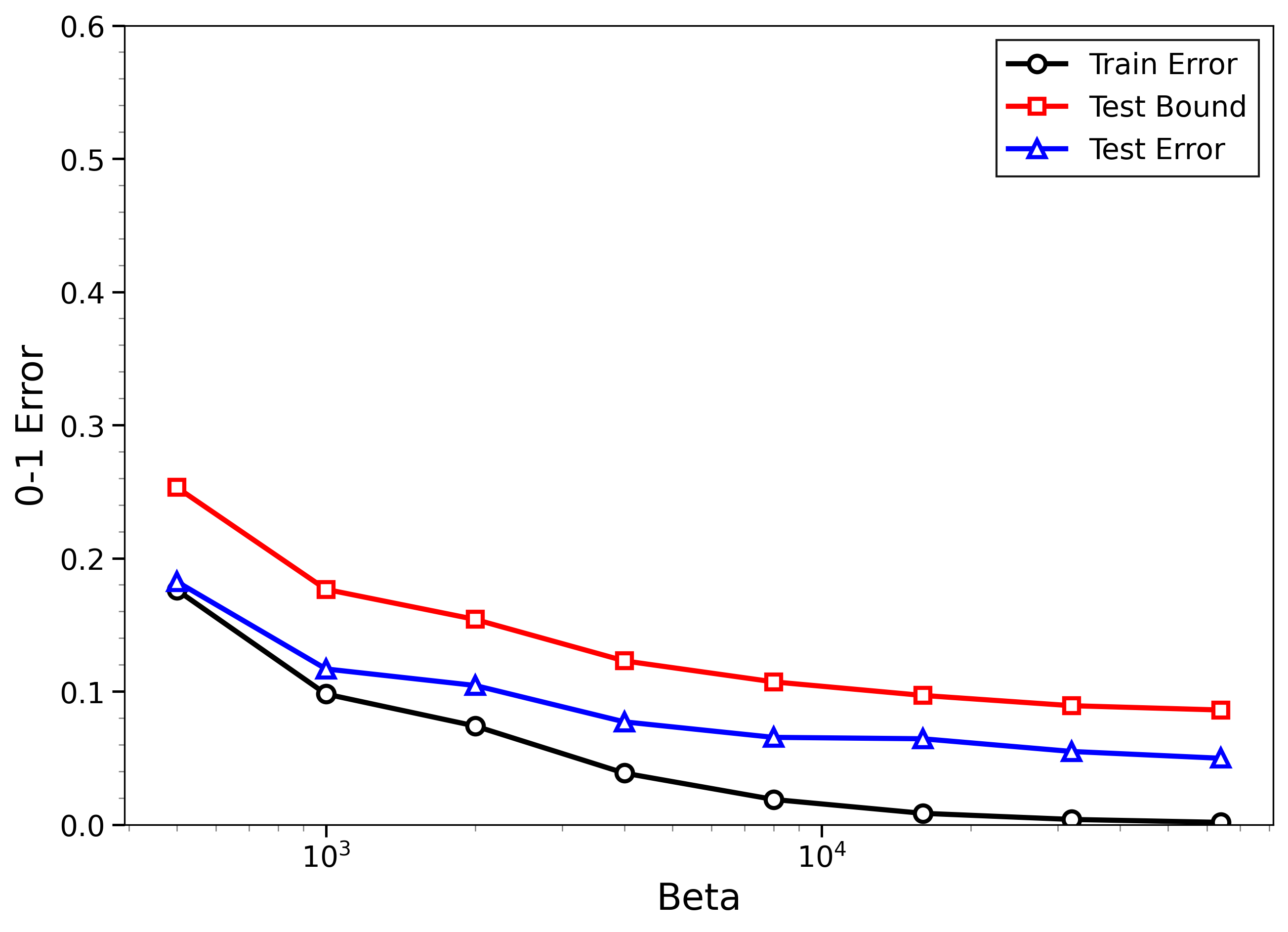
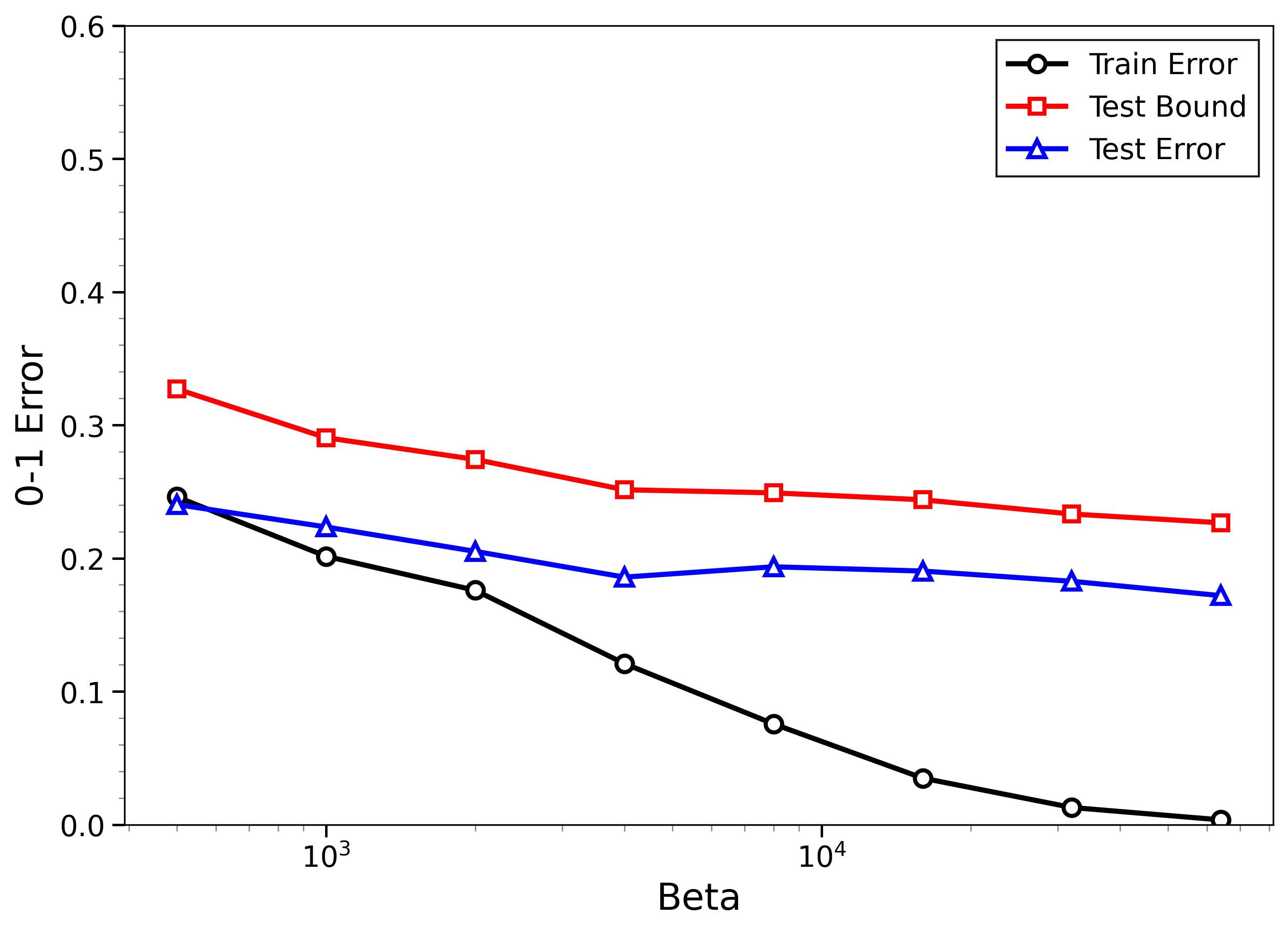
- The new bounds are nontrivial on real data:
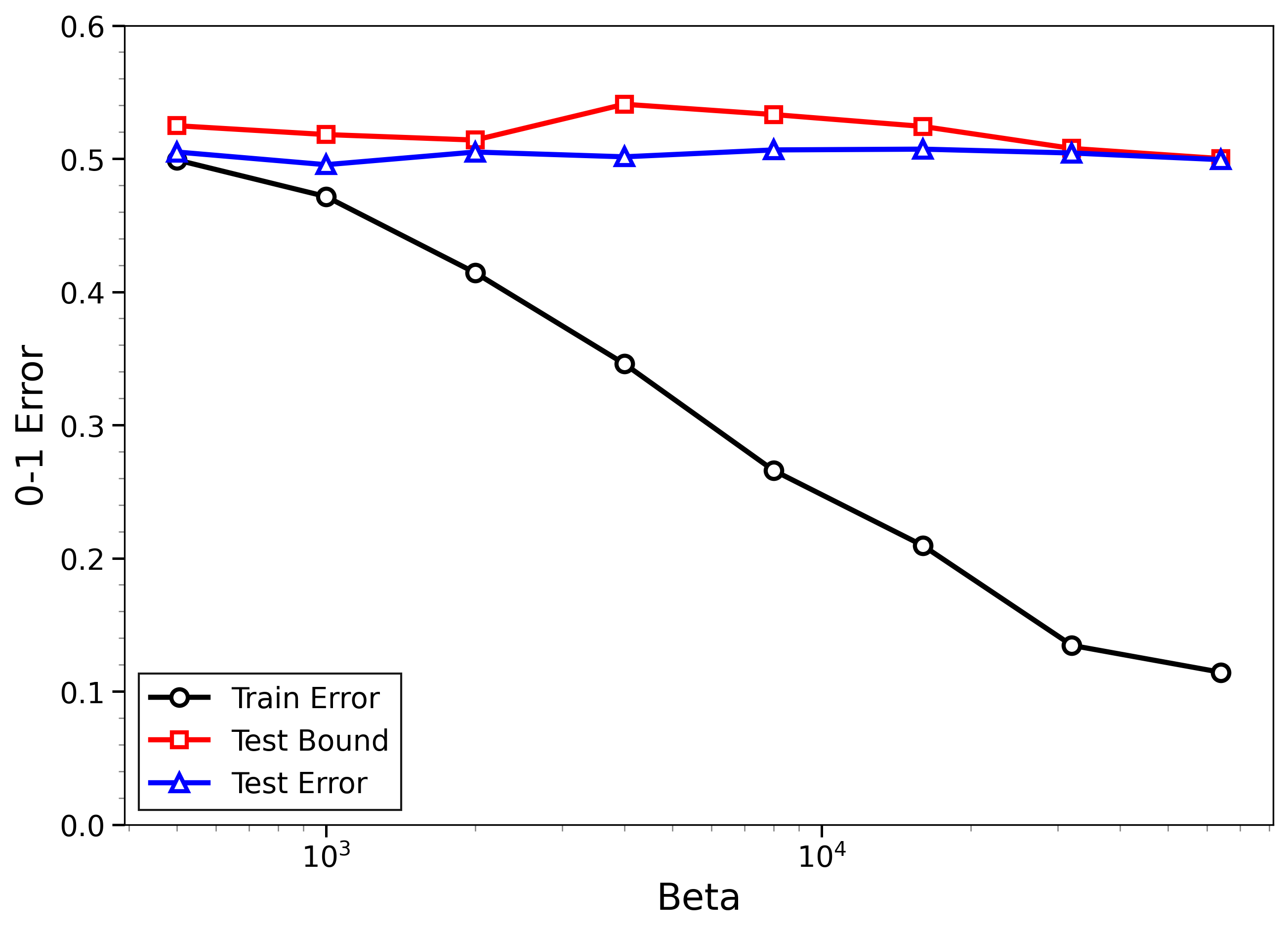
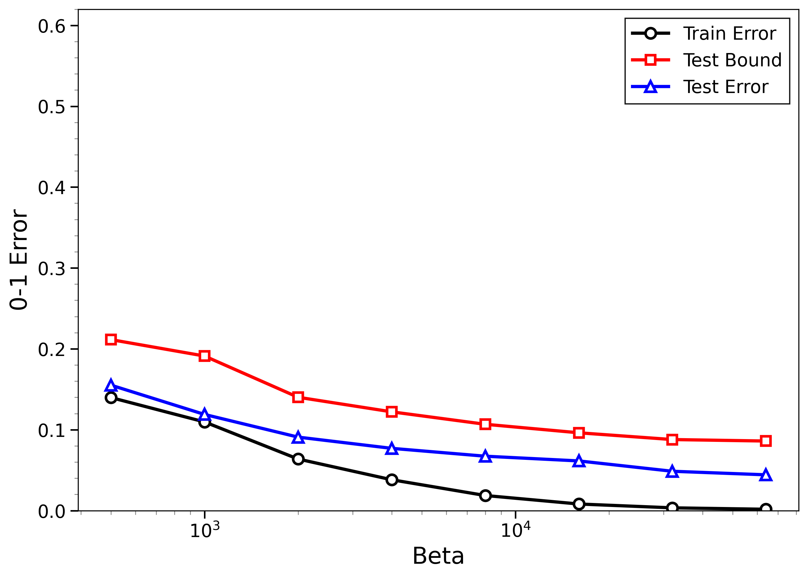
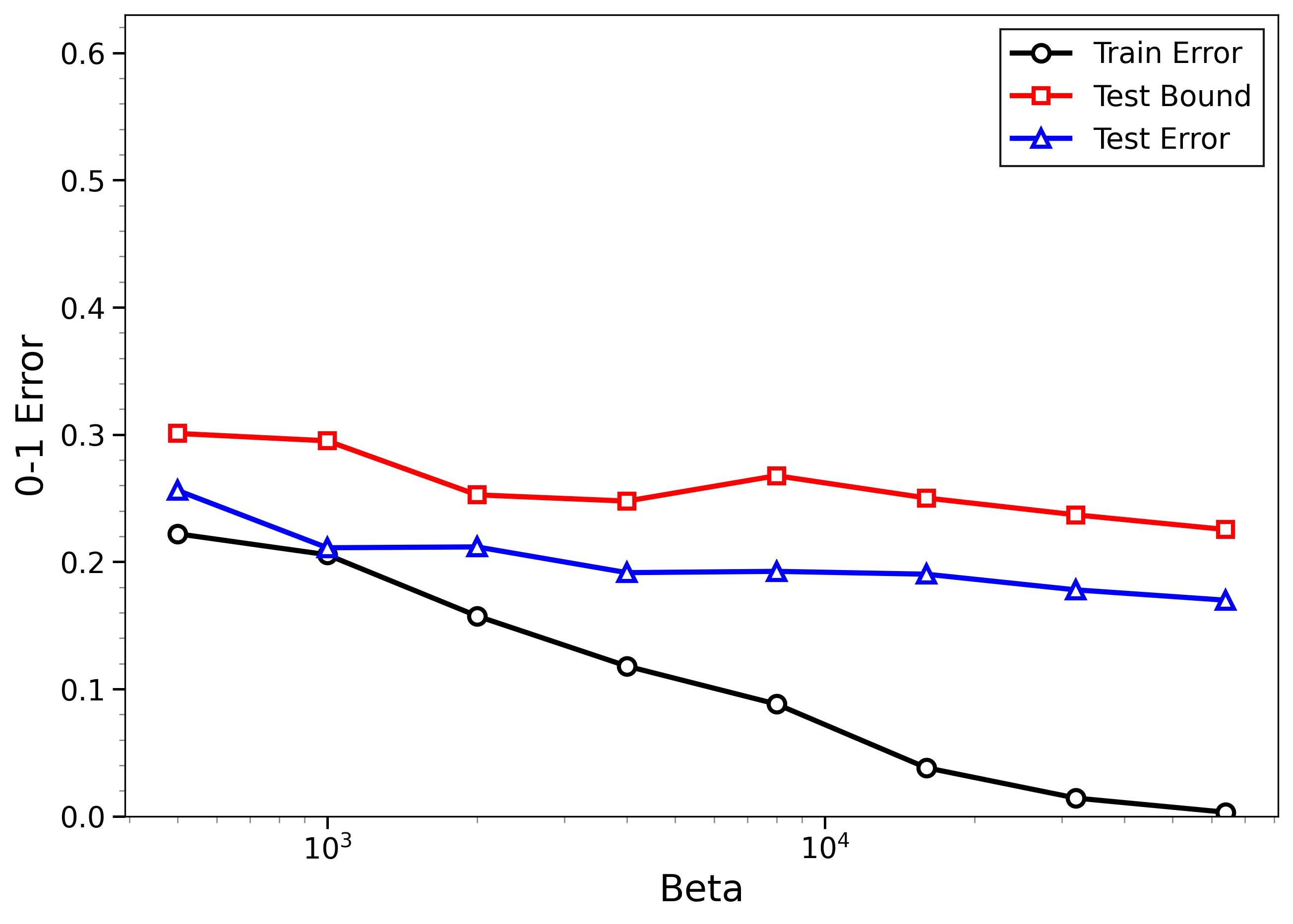
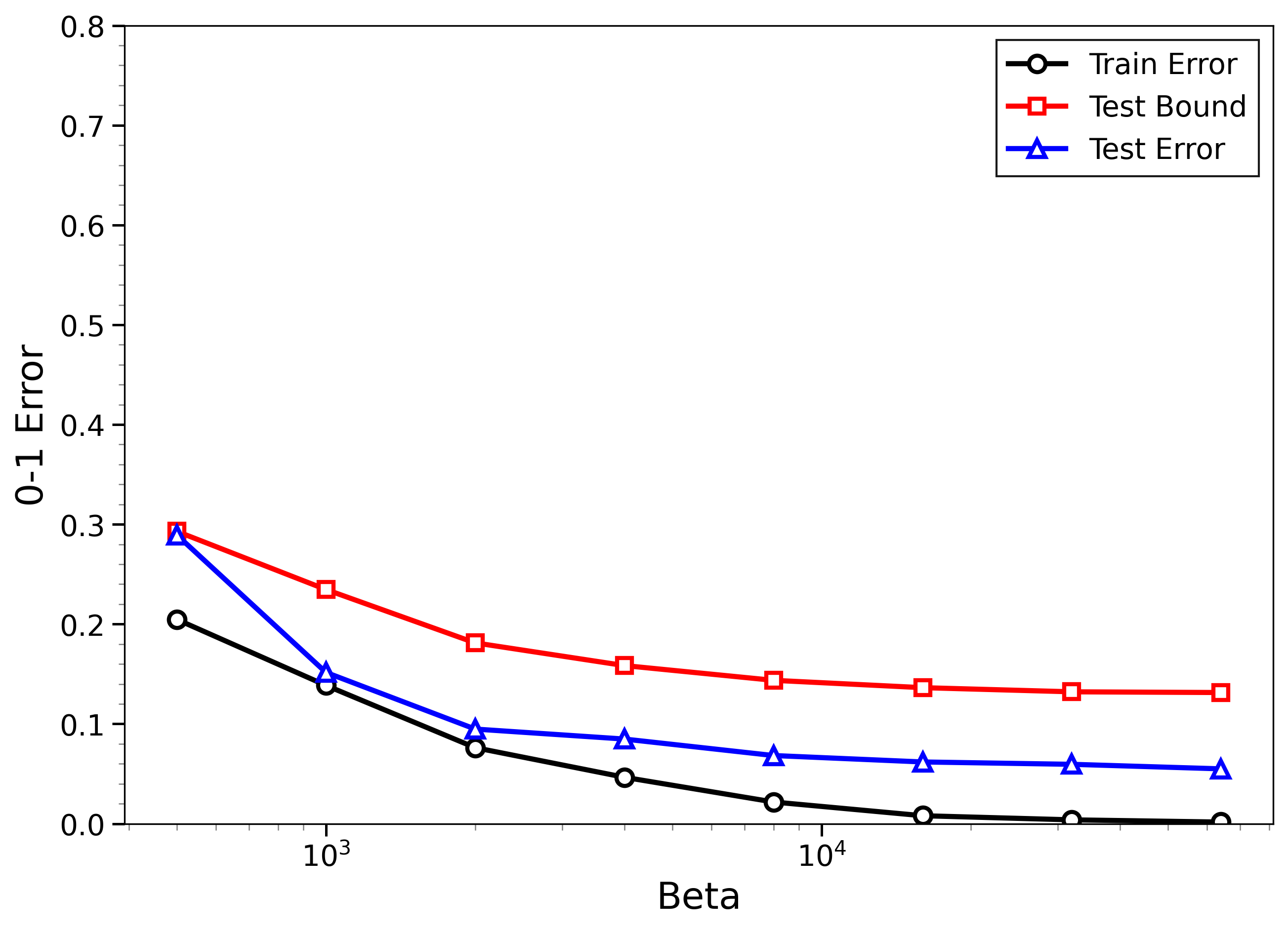
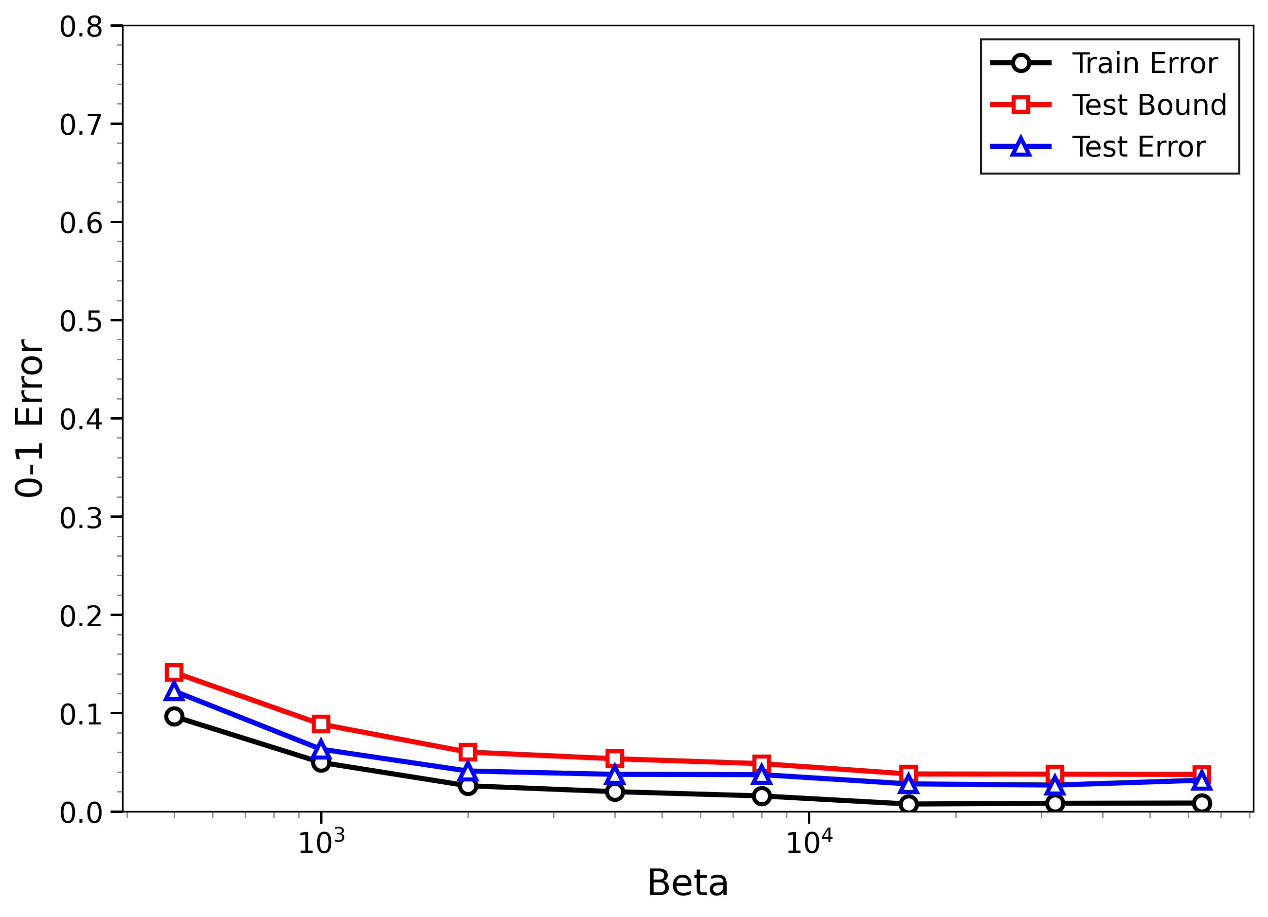
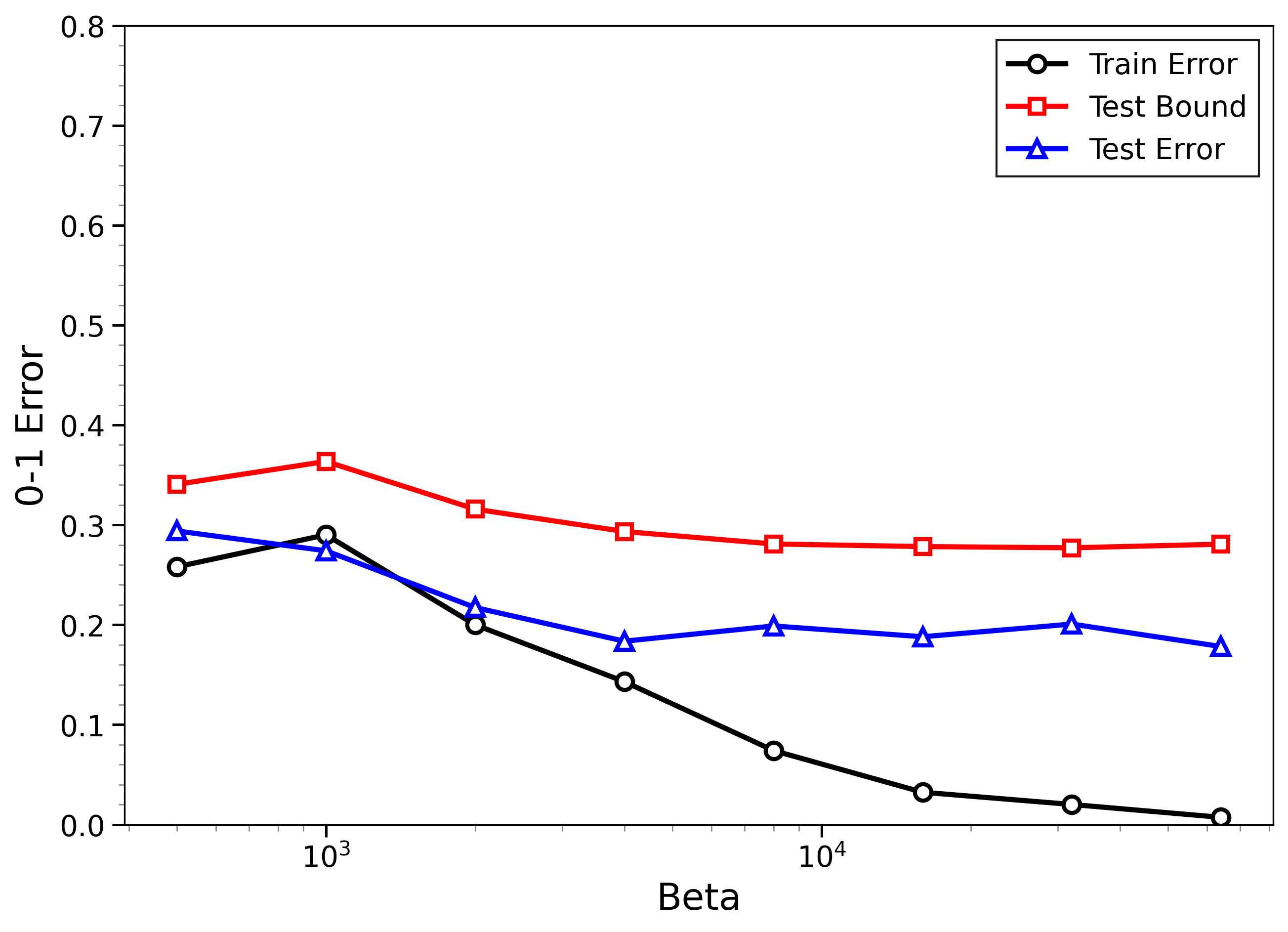
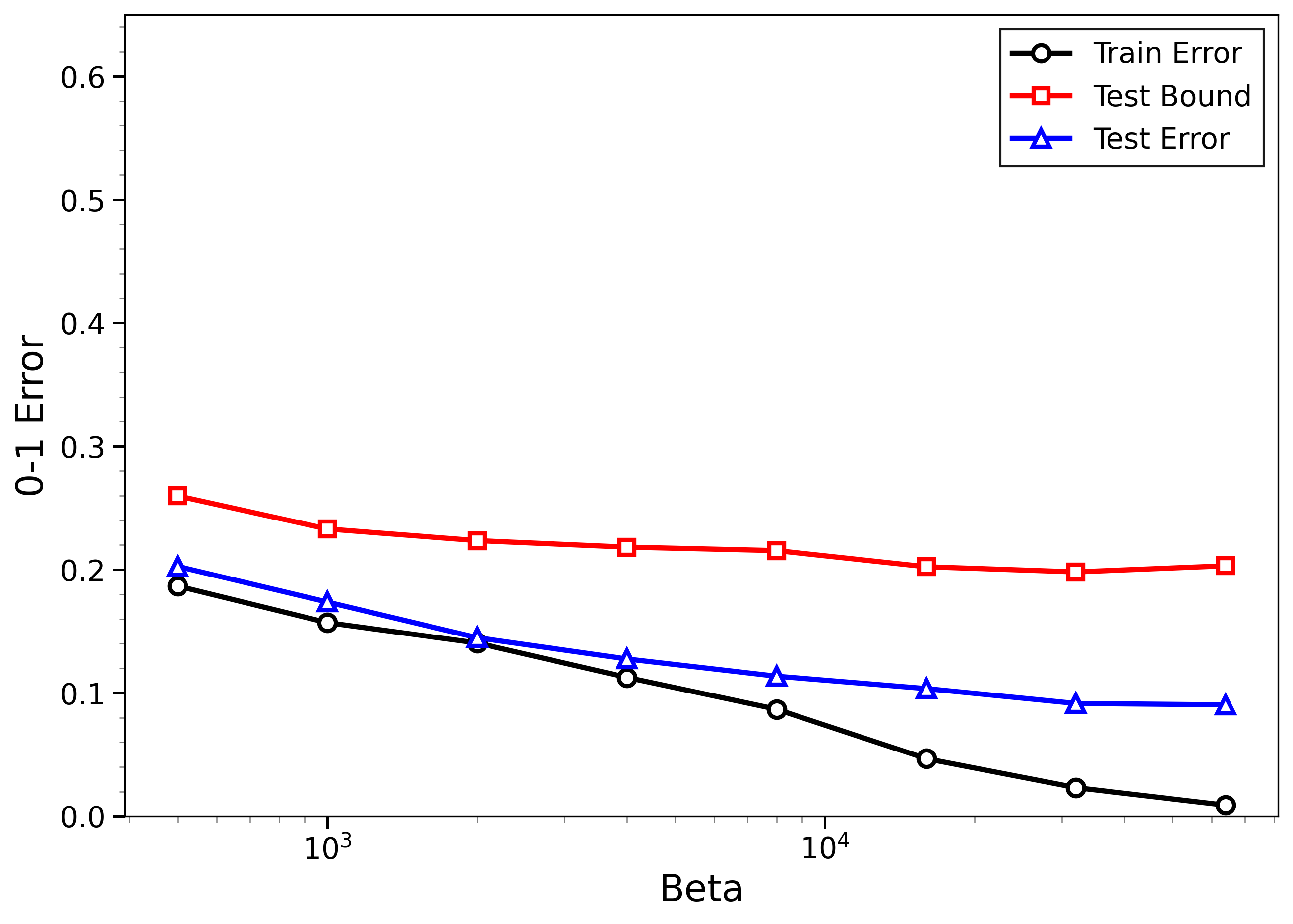
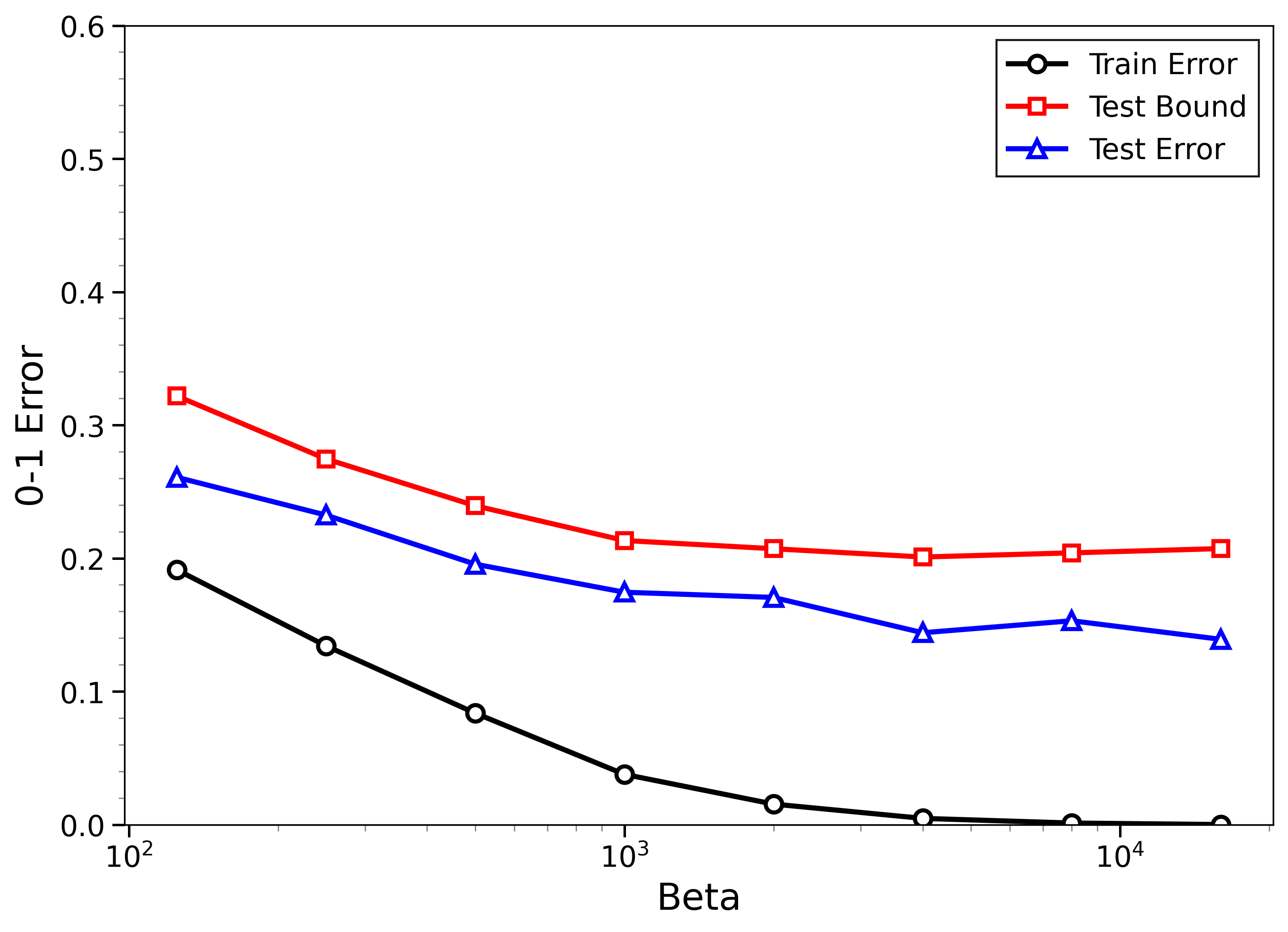
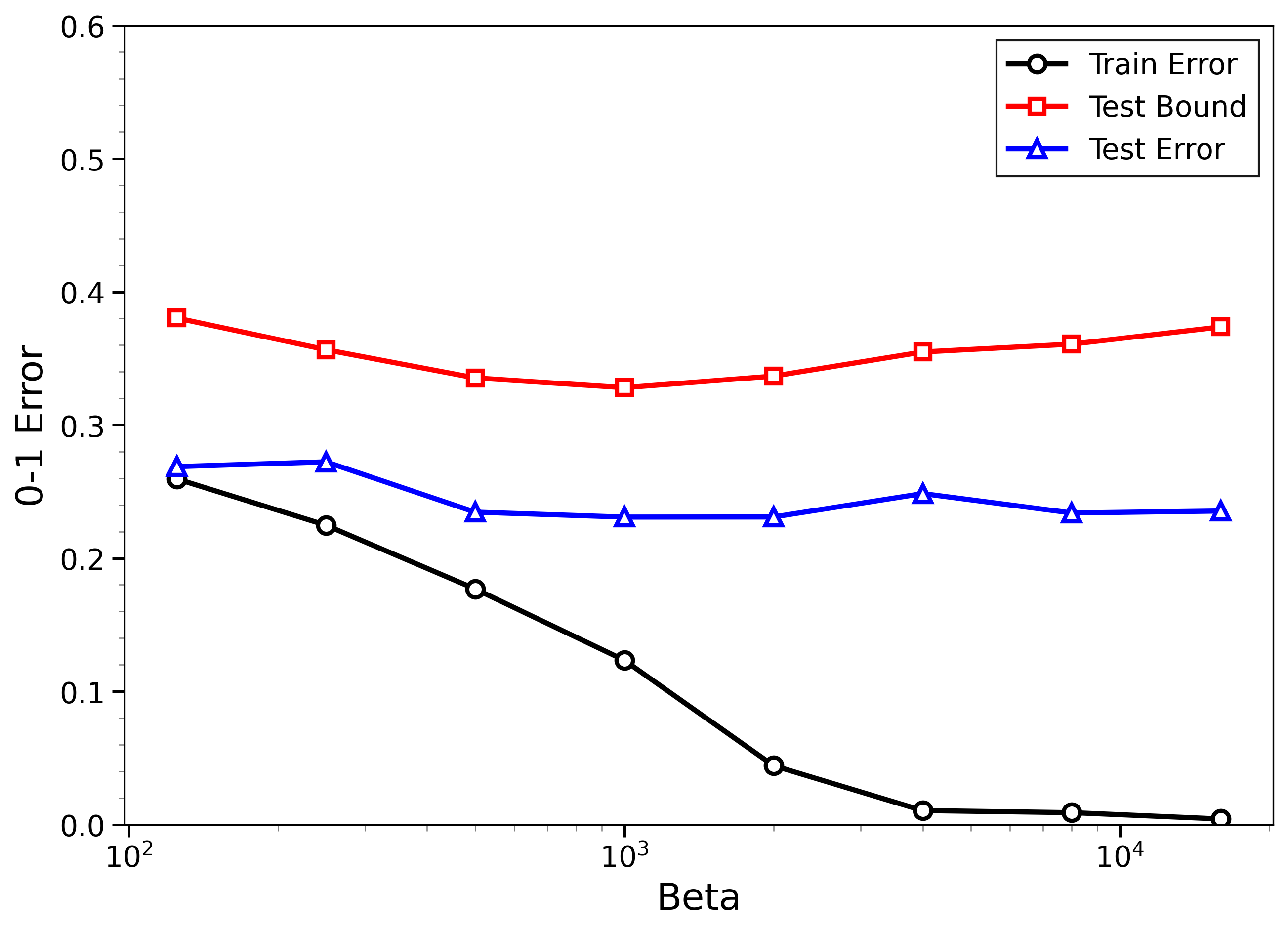
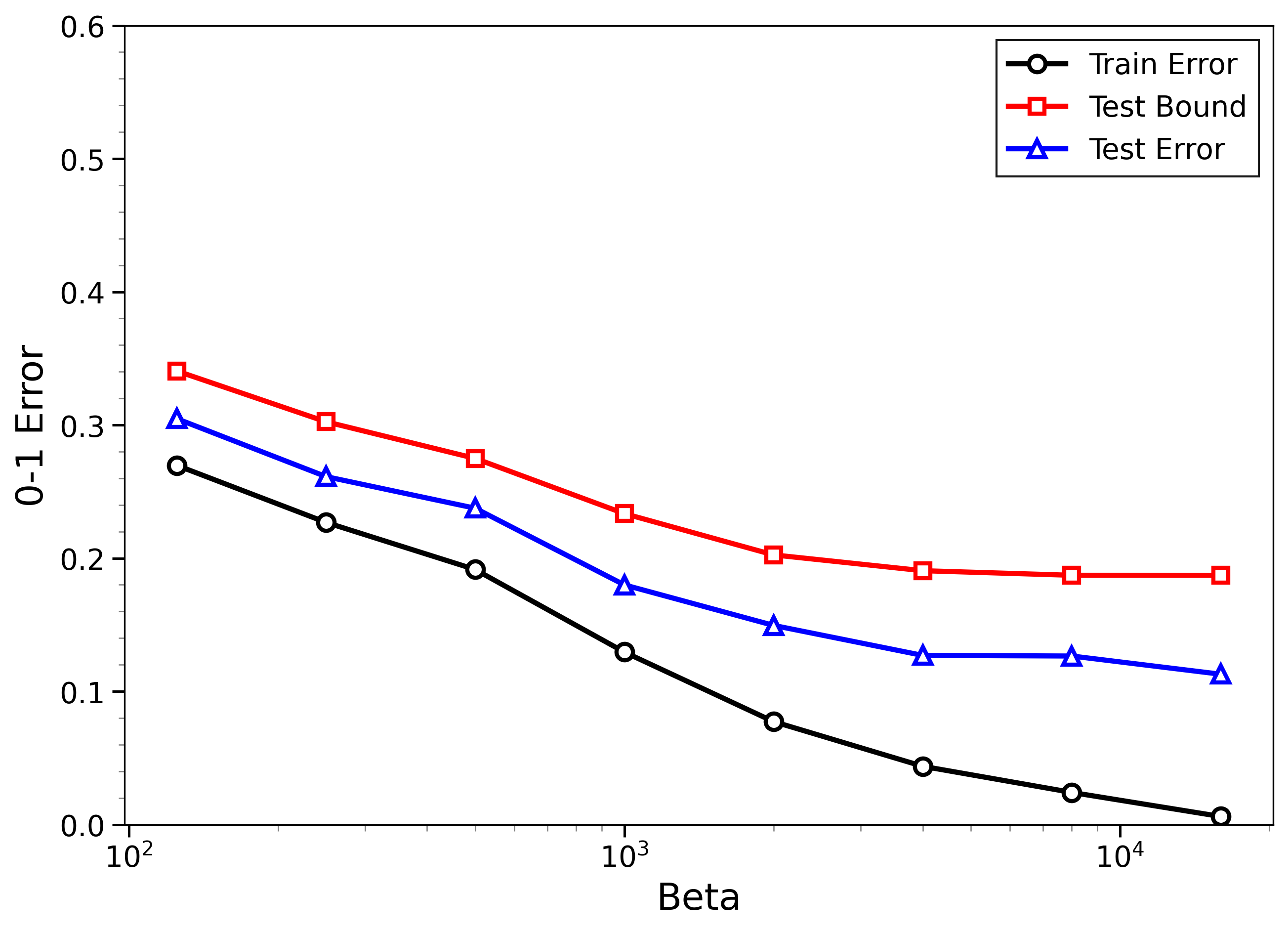
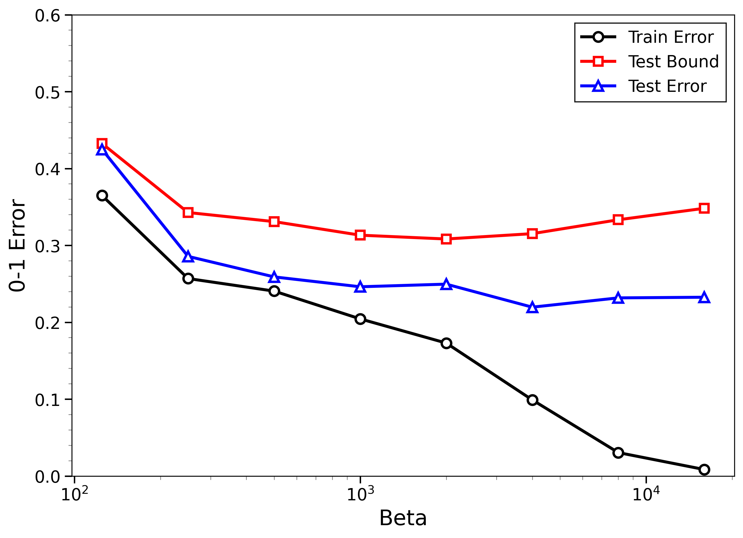
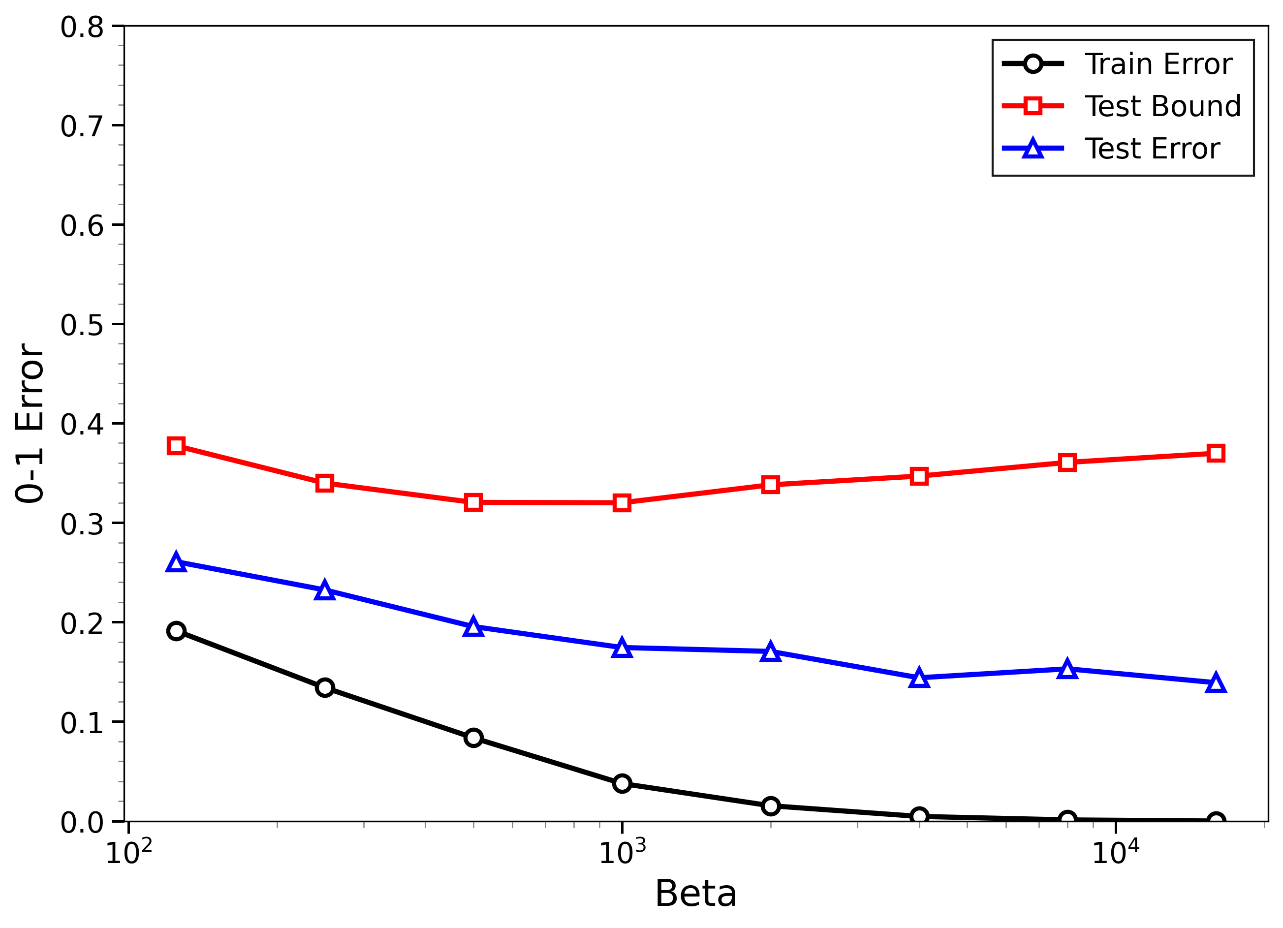
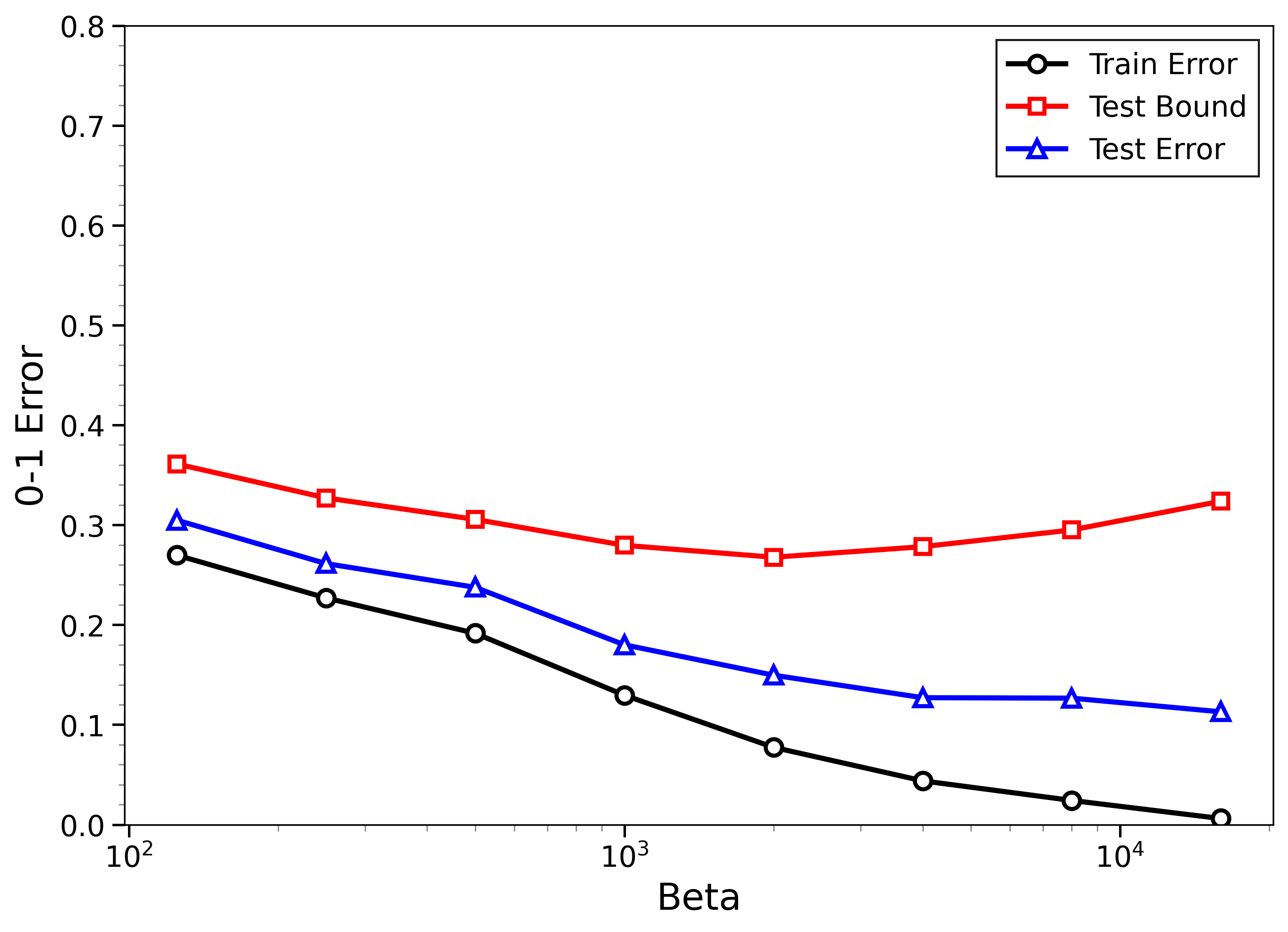
- On MNIST and CIFAR-10, the bounds give useful (not huge) upper limits on test error, even when the models can fit the training data almost perfectly.
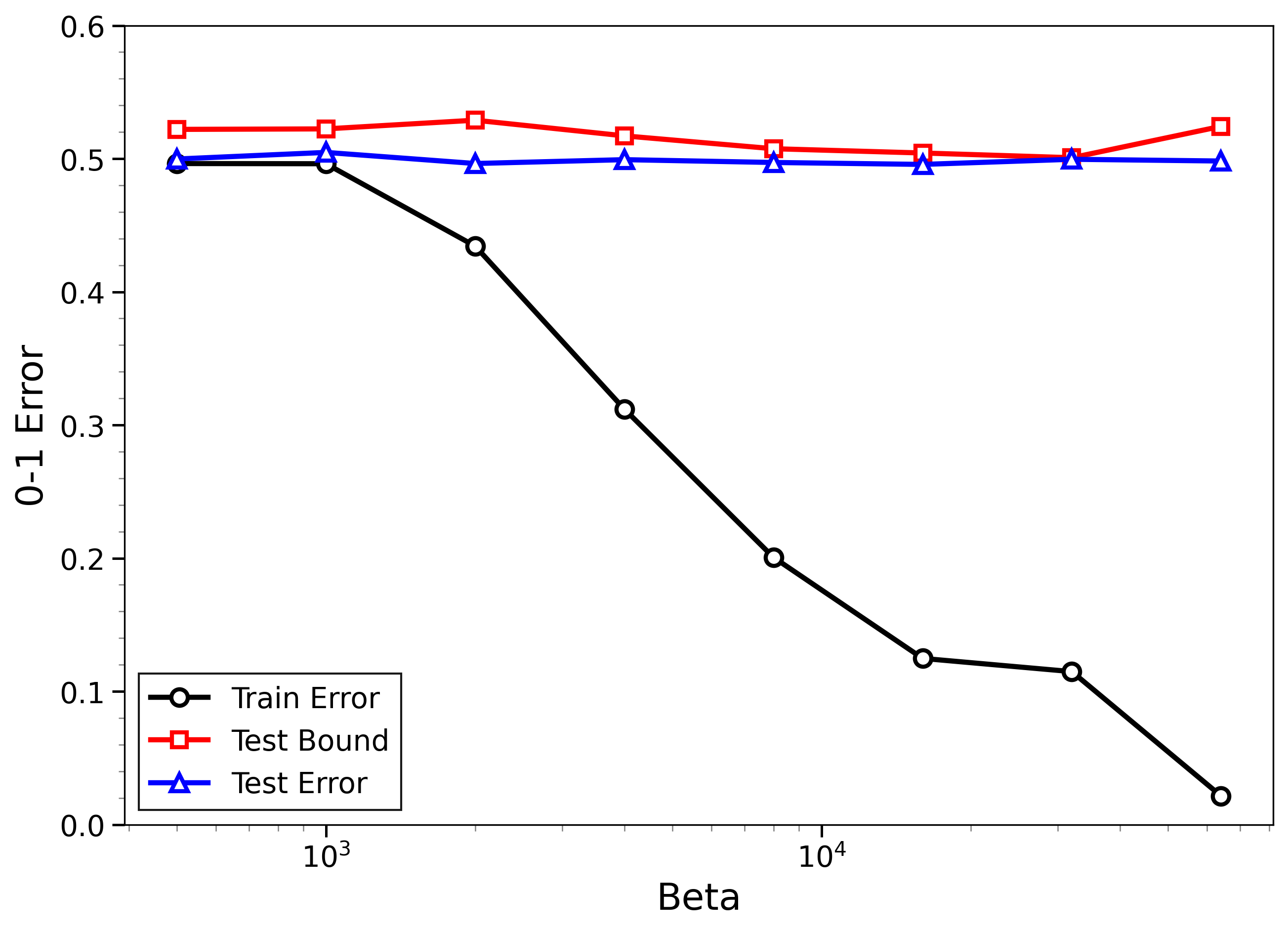
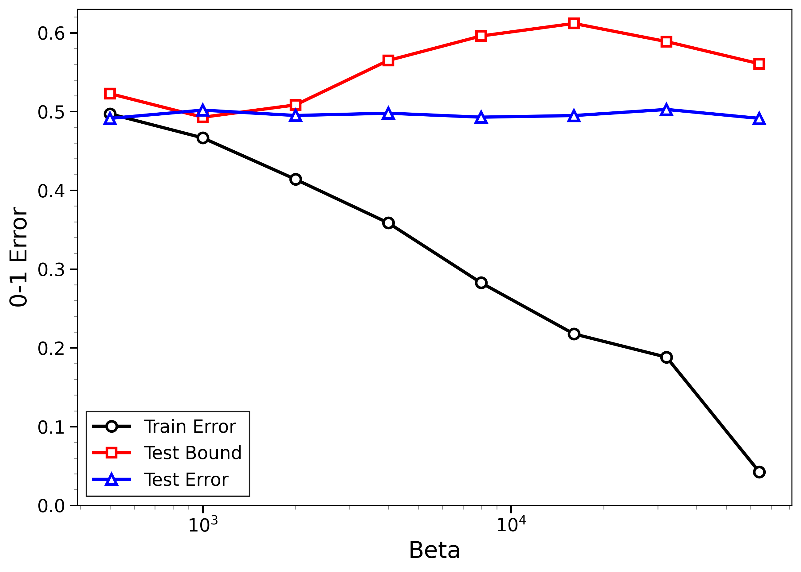
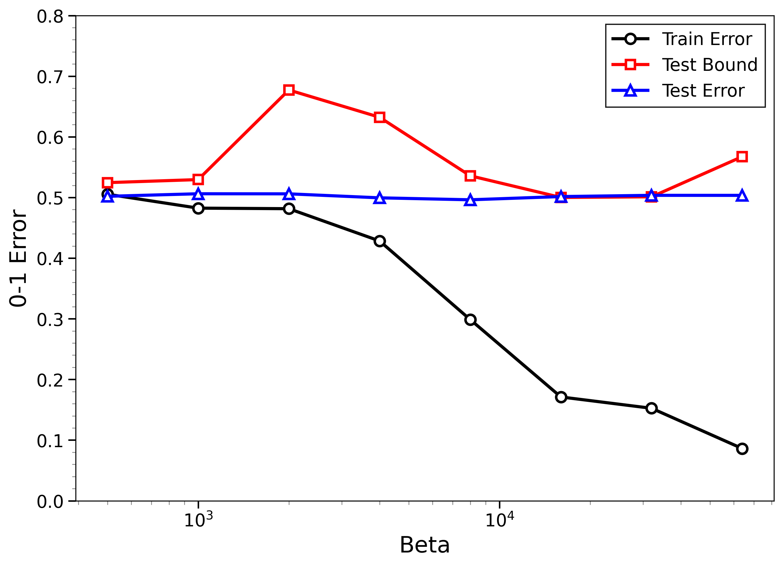
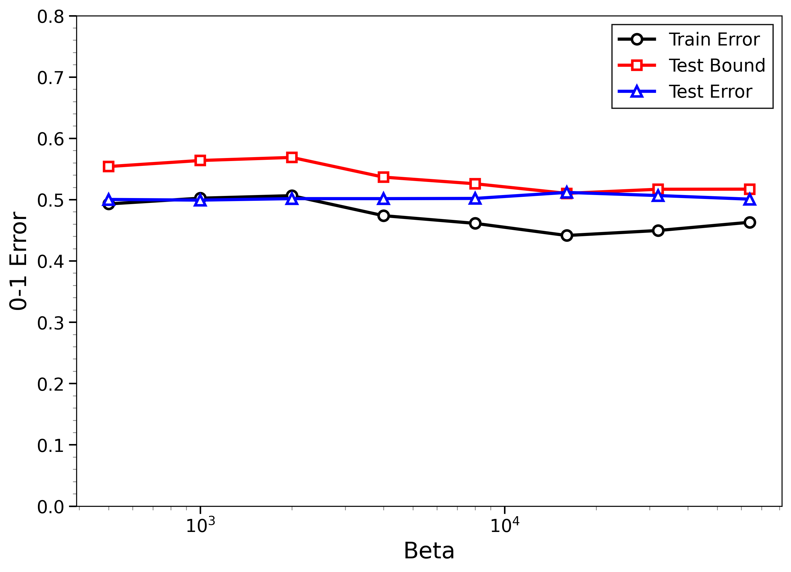
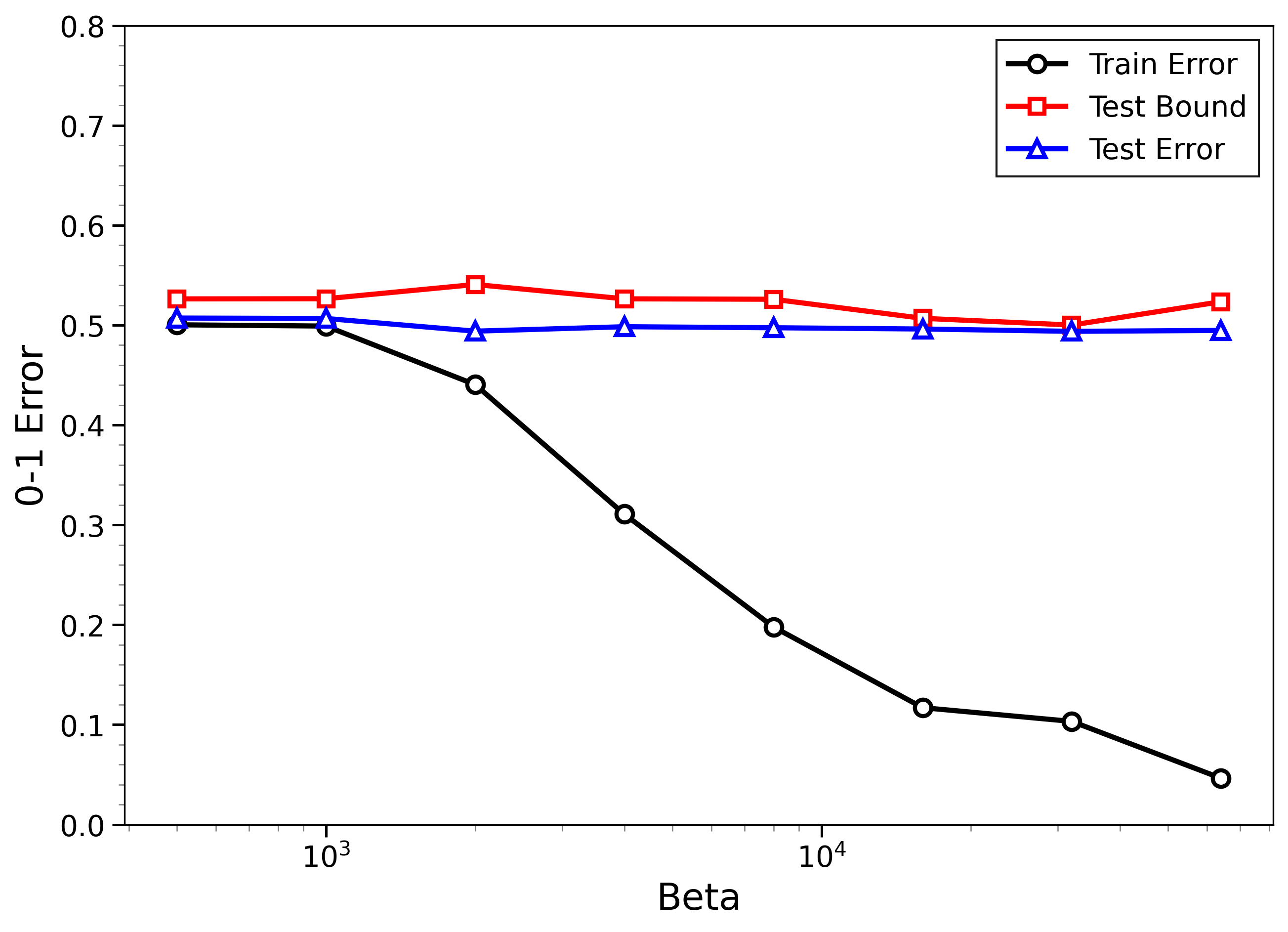
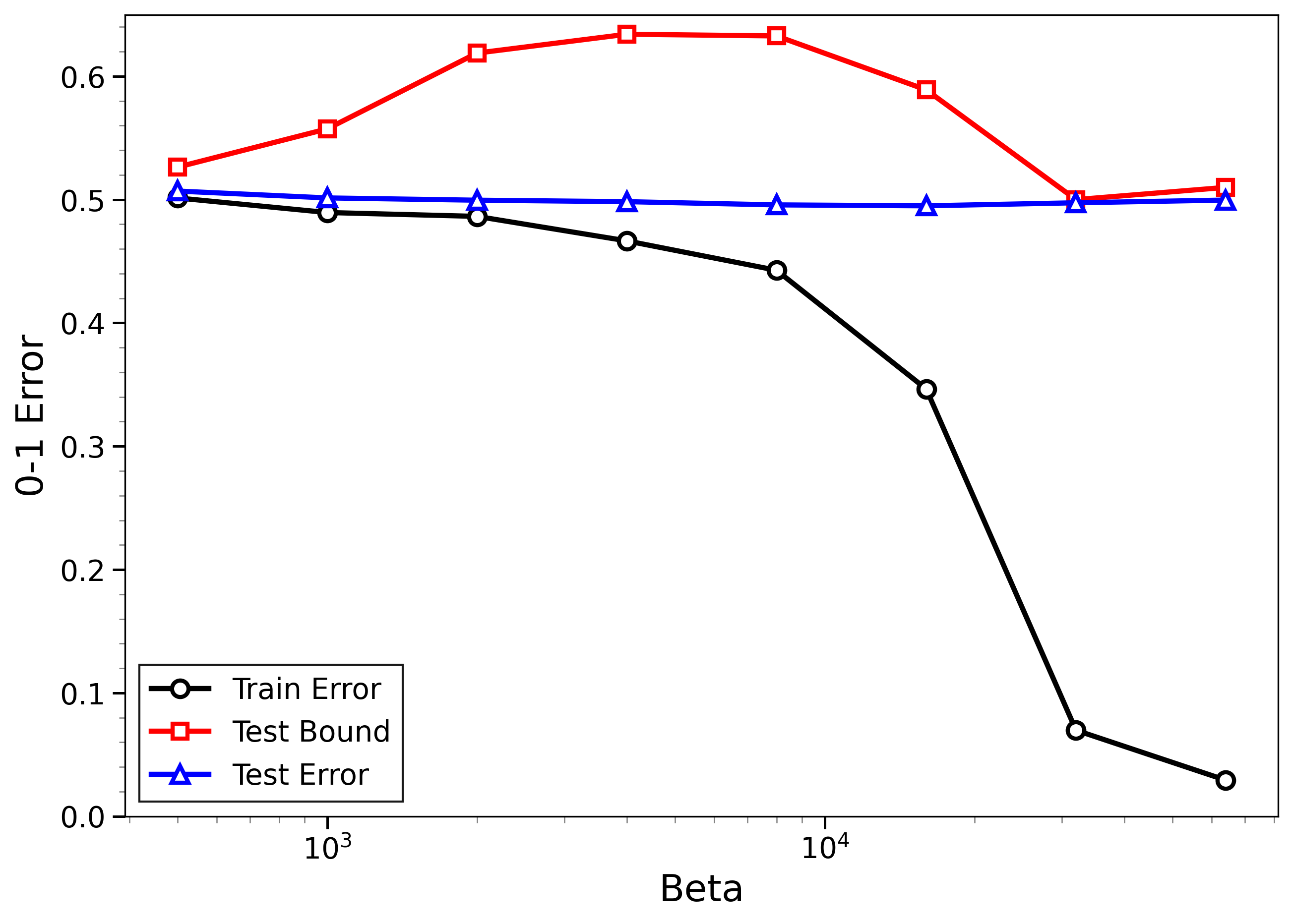
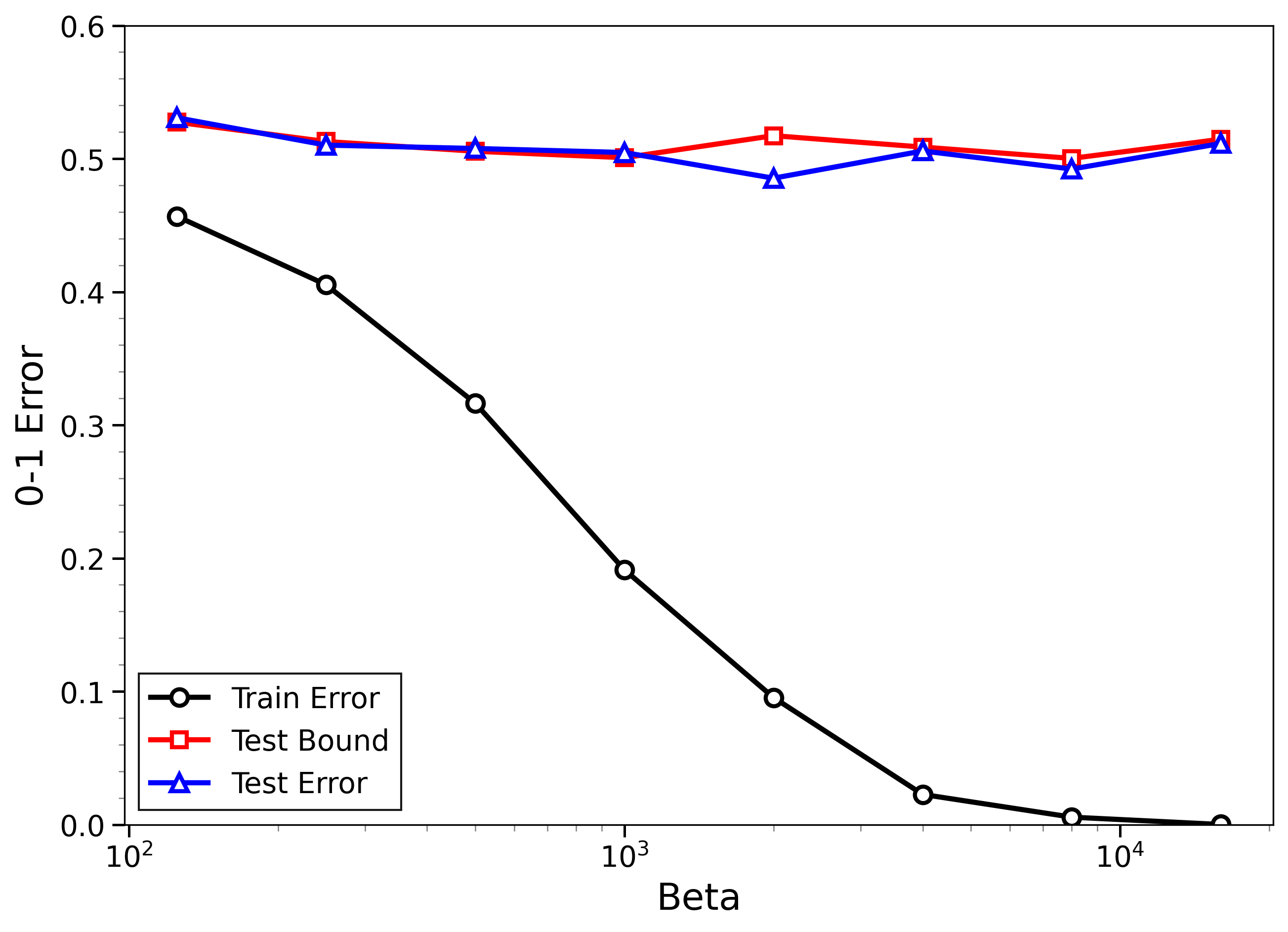
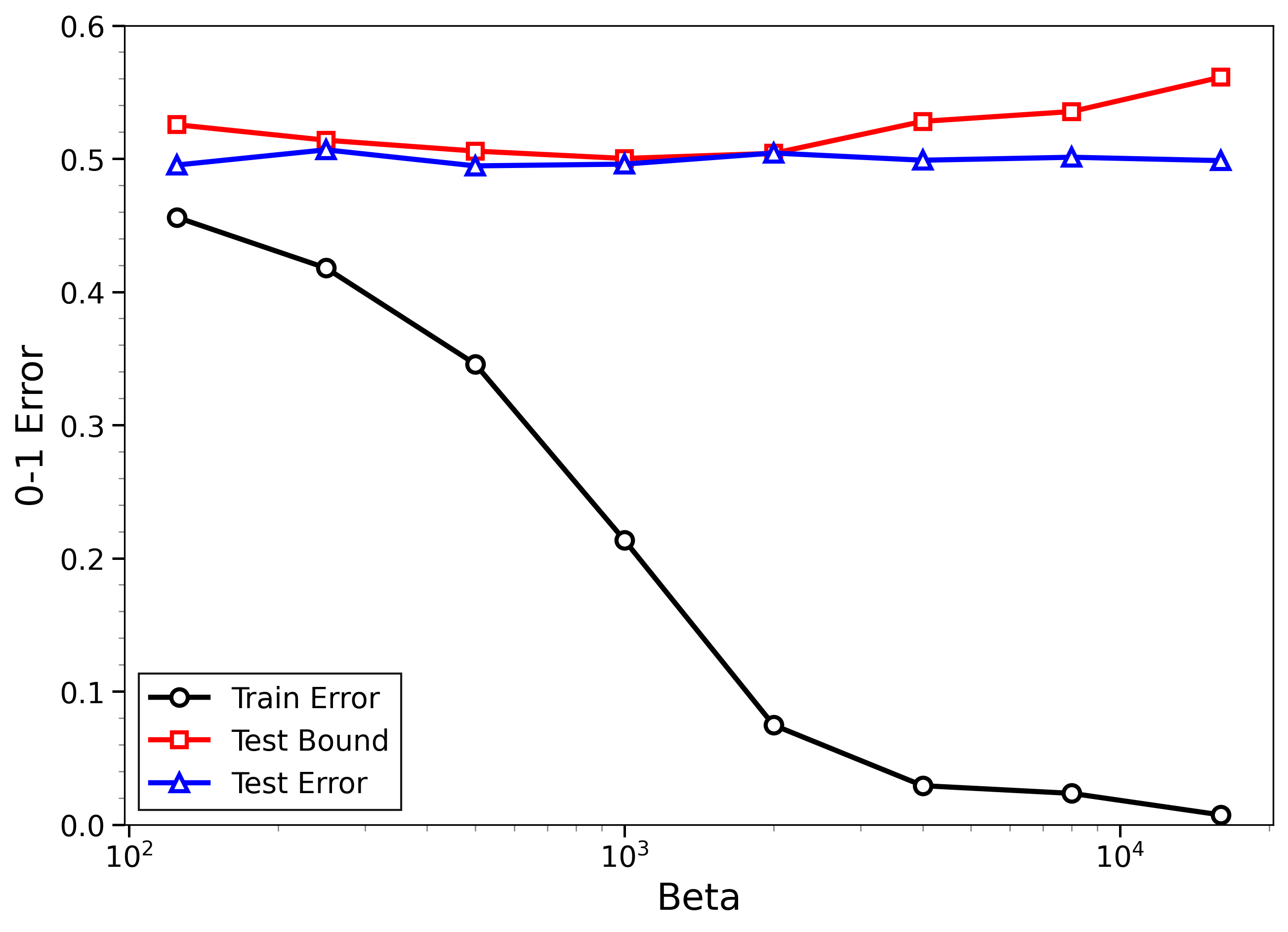
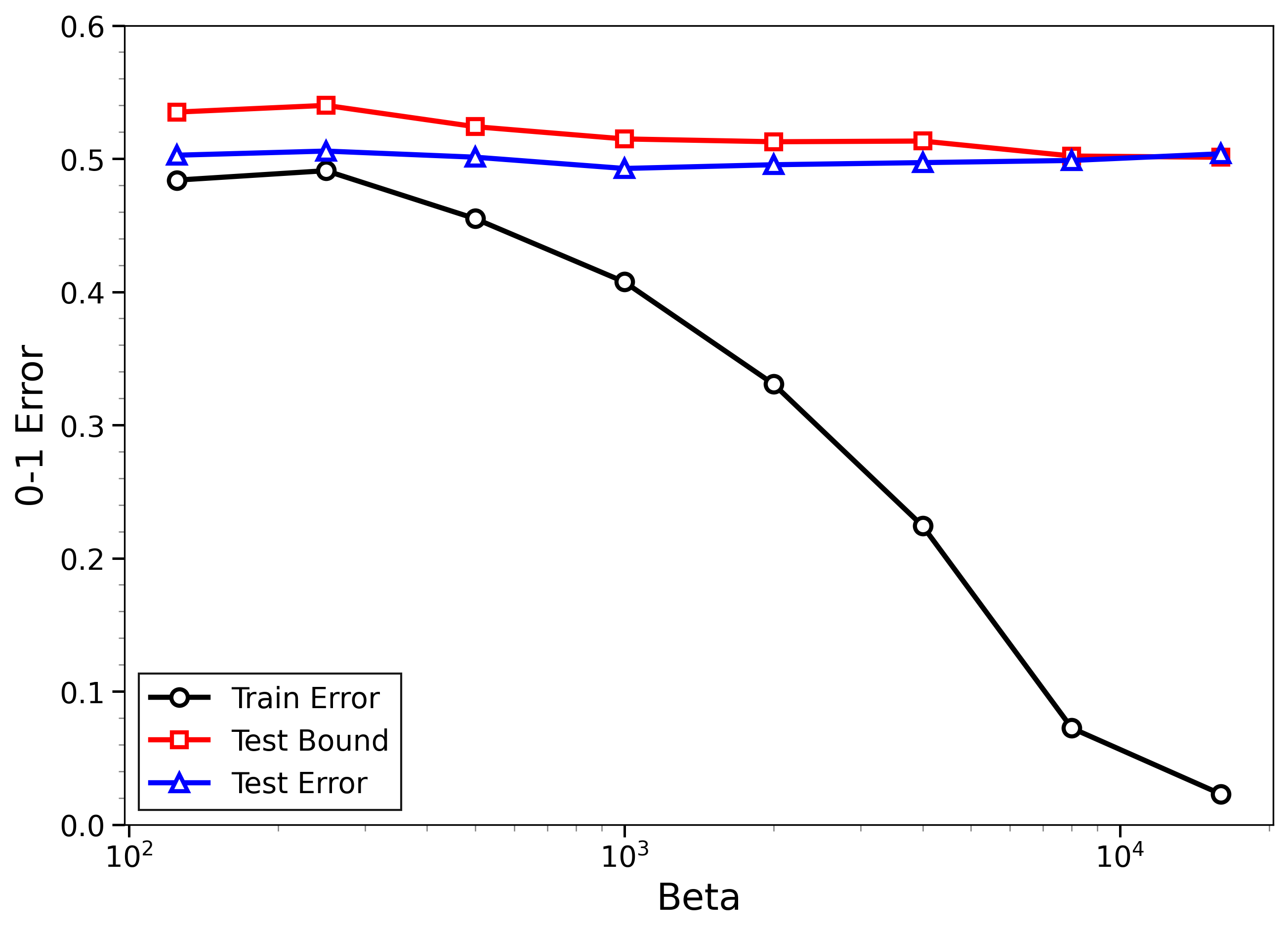
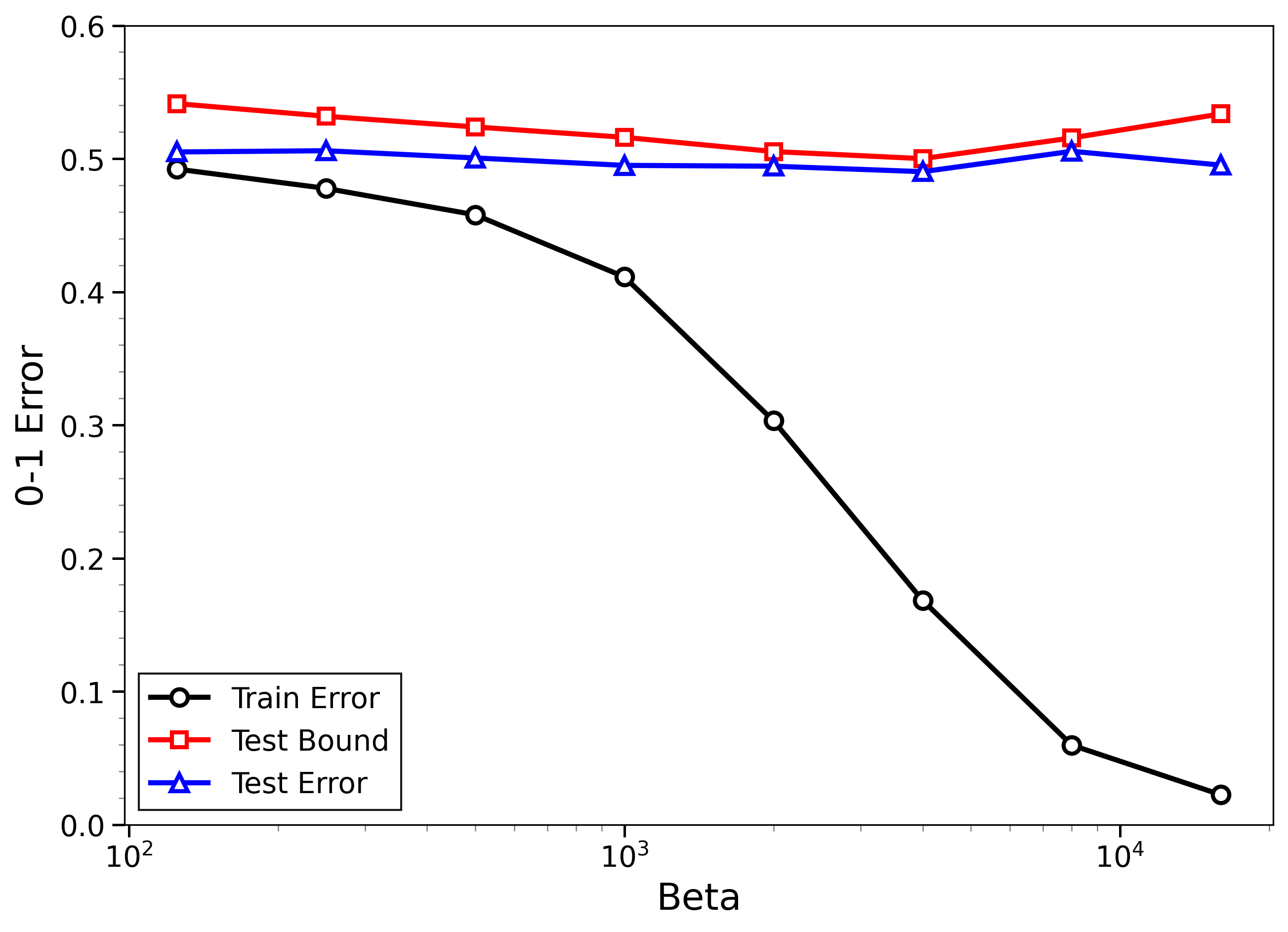
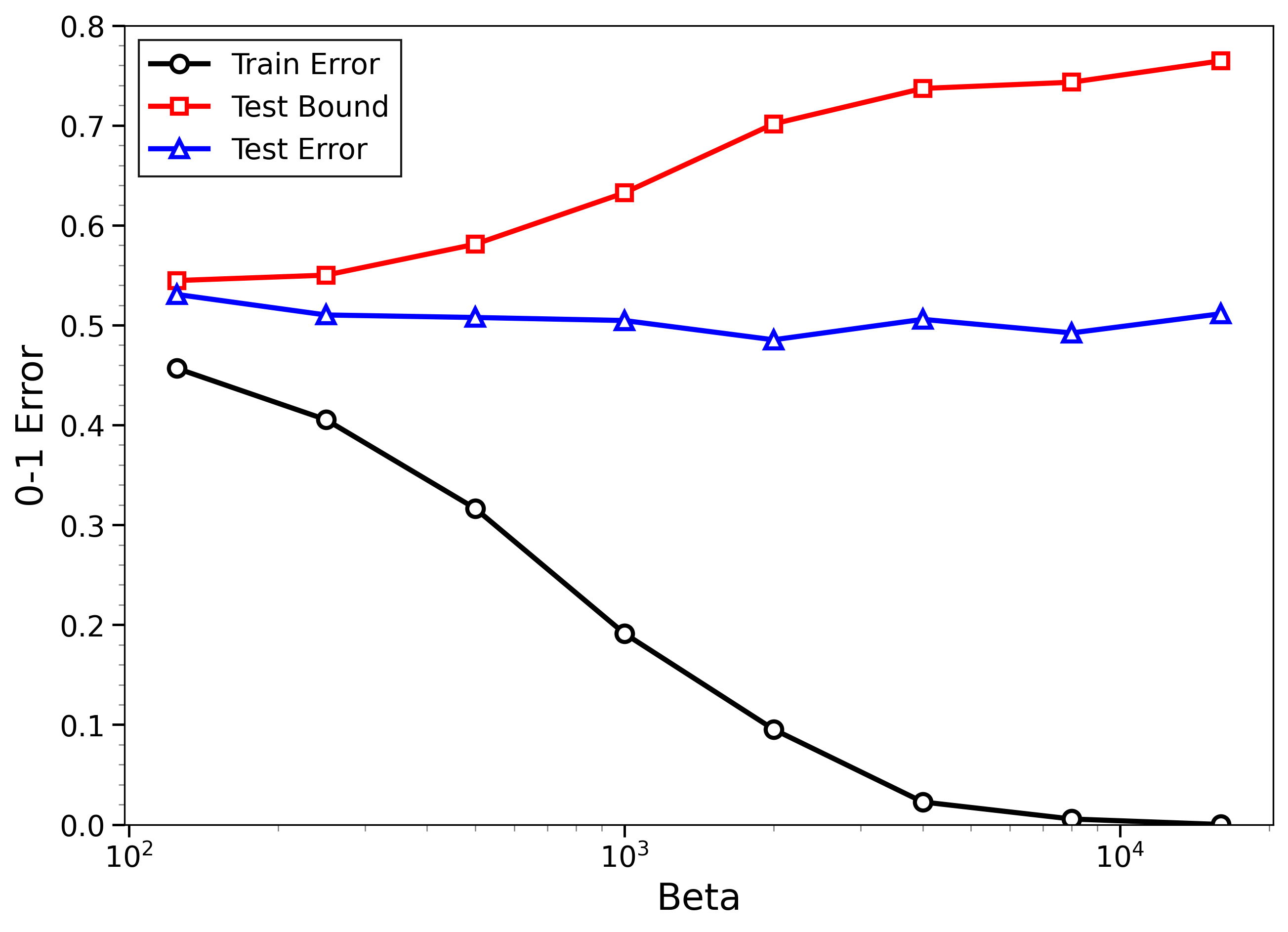
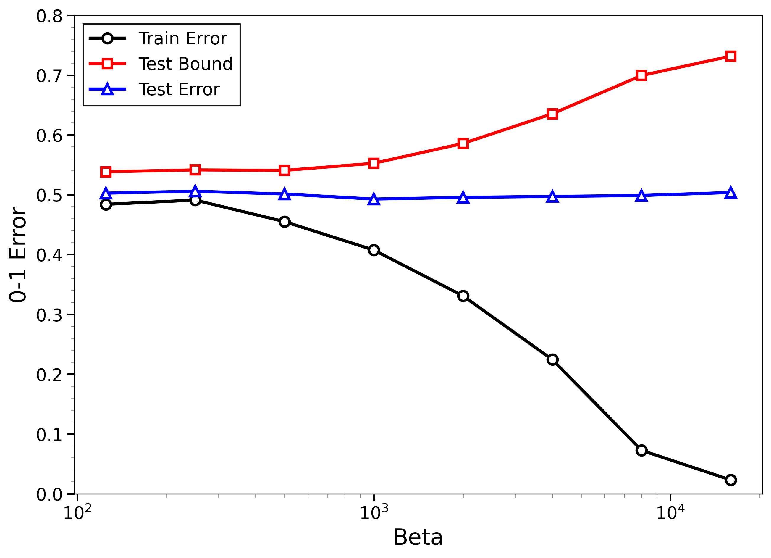
- The bounds behave correctly on random labels:
- When labels are randomized (an “impossible” task), training error gets very small, but the bounds correctly stay large, reflecting that test error will be bad. In other words, the method does not get fooled by memorization.
- High-temperature signals low-temperature generalization:
- They observe that if the training loss drops at higher temperatures (more exploration), this often predicts that the model will also generalize well at low temperatures (strong focus on the best-fit models). This connects an easy-to-measure regime to the harder, overfitting-prone regime.
- Approximate sampling is enough:
- Using LMC (like SGLD or ULA) with practical settings still produces bounds that match real outcomes, especially after the simple calibration based only on training data.
Why does this matter?
- Practical test-error guarantees for overpowered models:
- Modern models can memorize, so “low training error” alone isn’t a reliable sign of good generalization. This work provides data-dependent test-error bounds that stay meaningful even when models interpolate the training data.
- Bridges theory and practice:
- The method is theoretically grounded (PAC-Bayes + physics-inspired integral) and robust to using approximate samplers. With a single, training-data-only calibration, it becomes practical and surprisingly tight on real tasks.
- A diagnostic tool across temperatures:
- The “temperature ladder” view lets practitioners use safe, informative high-temperature measurements to anticipate generalization behavior in low-temperature, overfitting-prone regimes.
- Guidance for stochastic training:
- The stability results justify using common LMC-like training algorithms while still claiming test-error guarantees, helping connect sampling-based training with provable generalization.
In short, the paper introduces a way to predict test performance from training data alone for powerful models, shows the predictions are stable under practical sampling, and confirms on standard datasets that the bounds are both useful on real tasks and cautious on nonsense data.
Knowledge Gaps
Knowledge gaps, limitations, and open questions
Below is a concise, actionable list of what remains missing, uncertain, or unexplored in the paper’s theory and experiments.
- Practical validity of LSI and Hessian-boundedness assumptions: The bounds for LMC rely on a log-Sobolev inequality (LSI) with constant α and globally bounded Hessian (|∇²V| ≤ L), which are unclear or implausible for deep, nonconvex networks. Establish weaker, verifiable conditions (e.g., dissipativity outside compact sets, curvature conditions local to high-probability regions) that hold in realistic deep-learning settings and yield usable constants.
- Dimension- and step-size dependence: Theoretical approximation guarantees for ULA/LMC scale poorly with dimension d and require step sizes η that are orders of magnitude smaller than those used in practice. Derive nonasymptotic bounds with realistic η in high dimension (e.g., leveraging preconditioning, manifold Langevin, or covariance-aware priors) to reduce or remove prohibitive d and η dependencies.
- SGLD theory gap: Experiments use SGLD with constant step size, but the theory and stability results are given for ULA with full gradients. Provide explicit total-variation/Wasserstein error bounds for SGLD (including minibatch noise and constant steps) that can be plugged into the stability theorems to obtain end-to-end guarantees.
- Calibration heuristic lacks theory: The single calibration factor r, fitted using randomized labels, effectively rescales temperature and yields tight bounds empirically, but has no theoretical justification. Develop a principled calibration procedure with probabilistic guarantees (e.g., concentration of r, bias-variance trade-offs), and characterize its dependence on architecture, dataset, β-schedule, and step size.
- Diagnostics and error bars for ergodic means: The ergodic mean is approximated via ad hoc low-pass filters and a heuristic stopping rule. Provide mixing diagnostics (e.g., R-hat, integrated autocorrelation time) and finite-sample error bars for estimated expectations and Γν across β, especially under multimodality and nonstationarity.
- Single-draw bounds are impractical: The single-draw version requires exponentially tight TV approximations (in β and the range of F), making it unusable for realistic models. Develop alternative single-draw guarantees (e.g., via refined PAC-Bayes inequalities, heavy-tailed priors, Catoni-style robustification, or bounded-via-truncation strategies) that are compatible with practical LMC approximations.
- Temperature schedule optimization: The Γ functional requires expectations at a ladder of β values. There is no guidance on selecting the β grid. Design adaptive or optimized schedules (e.g., thermodynamic integration with control variates, tempering) that minimize computational cost while controlling discretization error in the integral representation.
- Unbounded loss handling: The method relies on bounded or Lipschitz losses (bounded-BCE or Savage loss) to keep moments finite. Extend the framework to unbounded but sub-exponential/sub-Gaussian losses (e.g., standard BCE) with explicit constants and practical moment controls, and quantify the impact of tail behavior on the bounds.
- Prior selection and preconditioning: A spherical Gaussian prior with fixed width σ is used. Investigate data-dependent or structured priors (layerwise scaling, diagonal/low-rank covariance, preconditioned Langevin) that improve both sampling accuracy and bound tightness, and provide selection rules with guarantees.
- Majority vote vs Gibbs average: The bound targets the Gibbs posterior expectation of the 0-1 loss; practitioners often deploy single models or majority votes. Analyze the gap between the Gibbs average, single-draw predictors, and ensemble majority votes, and derive corresponding bounds aligned with deployed predictors.
- Formalizing “high-temperature signals low-temperature generalization”: The paper argues qualitatively that small training errors at high temperature predict generalization at low temperature. Provide a rigorous theorem quantifying when and how high-temperature empirical performance controls low-temperature test error via the Γ functional, including explicit dependence on β-grid and sample size n.
- TV/Wasserstein stability constants: Stability theorems include additive errors proportional to εβk (TV or W2 discrepancies), but constants depend on unknown quantities (α, R, σ) and on m, M from boundedness/Lipschitz assumptions. Provide computable, data-driven proxies or upper bounds for these constants to turn the stability results into deployable certificates.
- Scaling and coverage of experiments: Experiments are limited to binary tasks, small sample sizes (2k–8k), and relatively small networks. Validate on multiclass tasks, larger datasets/models, and different architectures (e.g., CNNs, transformers), and report computational overhead and scalability of bound computation.
- Threshold choice for 0-1 conversion: Bounds for the 0-1 loss depend on choosing a threshold θ to map a surrogate to classification error. Provide a justified and data-driven method to select θ that preserves validity and yields tight bounds, including sensitivity analysis.
- Multimodality and initialization: Deep posteriors are likely multimodal; single-chain long runs may not traverse modes. Study the effect of initialization, use multiple chains/tempering, and quantify multi-modal bias in Γν and the resulting bounds.
- Adaptive β-level reuse: The method repeatedly approximates Gβk independently. Explore sample reuse across β (e.g., annealed importance sampling, bridging distributions) to reduce variance and compute, and quantify the induced bias/variance in Γ estimates.
- Non-iid data and beyond: The paper notes potential extension to Markovian data and U-statistics but does not develop it. Work out explicit bounds (moments, mixing conditions, constants) for non-iid settings and provide empirical validation.
- Tightening uncalibrated bounds: Uncalibrated bounds are sometimes nontrivial but still loose. Investigate variance-reduction techniques (e.g., control variates for loss estimates, MALA acceptance corrections, better discretization schemes) that provably tighten Γν without calibration.
- Sensitivity to σ and β: Provide a systematic study of how the prior width σ and the β-range affect bound tightness and stability, and derive guidelines for choosing σ and β to balance approximation accuracy and generalization tightness.
- Resource-aware guarantees: Quantify the trade-off between computational budget (steps, batch size, β-levels) and the tightness of the final bound, providing practitioners with prescriptions for how much computation is needed to reach a target certificate level.
Practical Applications
Immediate Applications
The following applications can be deployed now, leveraging the paper’s data-dependent generalization bounds for Gibbs posteriors and their stability under Langevin Monte Carlo (LMC) approximations.
- Generalization Bound Monitor in MLOps (software)
- What: Add a training-time diagnostic that computes an upper bound on test error for overparameterized models, even in the interpolation regime.
- How: Use bounded loss (e.g., bounded BCE or Savage loss), run ULA/SGLD across a temperature grid, compute the integral-representation-based functional Γ via ergodic means, and apply the paper’s calibration via randomized labels to produce bound curves as a function of β.
- Where: Integrate into CI/CD model training pipelines (e.g., PyTorch/TensorFlow plugin), and surface in Model Cards.
- Assumptions/dependencies: Requires approximate sampling via LMC (ULA/SGLD), bounded or Lipschitz losses, a Gaussian prior, sufficient compute for temperature sweeps, and a randomized-label calibration pass.
- Dataset and Label Quality Audit (software, education)
- What: Detect pathological data (e.g., random labels, heavy label noise) by contrasting small training error against high bound values.
- How: Run the same LMC pipeline on true labels and on a randomized-label copy; ensure the bound for random labels correctly upper-bounds test error (>0.5) while true labels yield tight bounds.
- Use: Early data curation during dataset construction or ingestion; supports identification of leakage or mislabeling.
- Assumptions/dependencies: Access to randomized-label variants of the training set; bounded loss and temperature sweep; ergodic mean approximations.
- Early-Temperature Generalization Diagnostic (software, robotics, energy, education)
- What: Use small training errors at high temperature (low β) as a signal of likely generalization at low temperature (high β).
- How: Perform a short β-sweep focusing on high-temperature regimes; check the initial slope and level of empirical loss; use as an architecture capacity check and early-stopping criterion.
- Use: Rapid triage for model capacity selection and training schedules.
- Assumptions/dependencies: Short LMC runs suffice; relies on the observed phenomenon that high-temperature performance predicts low-temperature generalization.
- Risk Reporting and Compliance for Regulated ML (healthcare, finance, public sector)
- What: Generate data-dependent PAC-Bayesian-style generalization certificates for overparameterized models, robust to interpolation.
- How: Attach bound curves and calibration details to Model Cards or compliance dossiers; use bounds to justify deployment thresholds and risk controls.
- Assumptions/dependencies: Choice of prior and loss; LMC approximations; reproducible β-sweep and calibration procedure; sufficient documentation for auditors.
- Model Selection and Hyperparameter Tuning (software)
- What: Select architectures, priors (σ), and β-schedules that minimize the bound rather than only optimizing validation metrics.
- How: Compare Γ-derived bounds across candidate models/priors and temperature schedules; prefer configurations with tighter bounds on expected 0–1 loss.
- Assumptions/dependencies: Stable LMC runs; bound computation under bounded loss; calibration factor derived from the training set.
- Overfitting Defense and Data Poisoning Detection (software, security)
- What: Flag suspicious training runs where training error collapses but bounds stay high, indicating possible poisoning/backdoors or mismatch between train and test distributions.
- How: Monitor training-vs-bound divergence during β-annealing; trigger forensic checks when patterns mirror randomized-label behavior.
- Assumptions/dependencies: Continuous bound computation; baseline from randomized-label calibration; controlled training environment.
- Teaching and Reproducible Research Assets (academia)
- What: Provide code snippets and lab exercises showing PAC-Bayes + Γ bounds across β with LMC approximation and calibration.
- How: Adopt the open repository workflow to produce bound plots for standard benchmarks (MNIST, CIFAR-10); include randomized-label calibration demos.
- Assumptions/dependencies: Moderate compute; standard ML frameworks; didactic datasets.
Long-Term Applications
The following applications require further research, scaling, or development to become robust and widely deployable.
- Certified LMC Training Algorithms (software, robotics, healthcare)
- What: Develop LMC/ULA/SGLD variants with provable closeness to Gibbs posteriors in W2/TV, enabling reliable single-draw bounds without heavy calibration.
- How: New step-size schedules, coupling methods, and dissipativity/LSI verification tools; runtime certificates for approximation quality.
- Dependencies: Practical estimation or control of LSI constants; scalable verification protocols; efficient mixing in high dimensions.
- Bound-Aware Optimizers and Training Schedules (software, energy)
- What: Optimizers that directly minimize Γ or its bound proxies, with temperature annealing guided by high-temperature generalization signals.
- How: Adaptive β-schedules, prior tuning (σ), and loss shaping to improve bound tightness; incorporate into AutoML loops.
- Dependencies: Fast bound estimation loops; compatibility with standard training regimes; robust calibration across tasks.
- AutoML Guided by Generalization Bounds (software)
- What: Architecture/prior/hyperparameter search driven by bound metrics rather than validation loss alone, especially in small-sample or high-noise settings.
- How: Multi-objective AutoML that includes Γ-based bounds as a first-class optimization objective; temperature sweep and calibration integrated.
- Dependencies: Efficient LMC approximations at scale; caching and reuse of β-sweep results; low overhead for large model families.
- Safety-Critical Deployment Gating (healthcare, finance, robotics)
- What: Formal thresholds on bounds for mission-critical ML systems; models cannot ship unless bound criteria are met across β-sweeps.
- How: Organizational policies and tooling that enforce “generalization gate” checks; integration with risk management frameworks.
- Dependencies: Regulatory buy-in; standardized bound computation procedures; domain-specific loss and prior choices validated.
- Standards and Policy for Generalization Guarantees (public sector, policy)
- What: Include empirical PAC-Bayesian-style bounds in AI assurance standards and procurement requirements (e.g., EU AI Act compliance guidance).
- How: Reference implementations and audit-ready documentation; harmonized reporting (Model Cards + bound plots + calibration details).
- Dependencies: Consensus on acceptable priors/losses/β-sweeps; auditor training; benchmarks for diverse domains (classification, regression, multi-class).
- Bound-Guided Data Valuation and Active Learning (software, education)
- What: Use bound sensitivity to identify valuable data points or mislabeled samples; drive labeling budgets and active acquisition.
- How: Analyze how Γ and test-error bounds shift with incremental data; choose queries that most tighten bounds.
- Dependencies: Efficient recomputation or incremental updates of bounds; robust behavior under non-iid and Markovian data (as hinted by the paper’s extensions).
- Foundation Models Auditing and Fine-Tuning Controls (software)
- What: Adapt Γ-based bounds to large-scale pretraining/fine-tuning, providing generalization assurances when labels are scarce and models interpolate.
- How: Scalable LMC approximations or surrogate measures; temperature schedules for fine-tuning phases; bound-aware early stopping.
- Dependencies: Practical approximations for very high-dimensional parameter spaces; new bounded losses compatible with large-model training.
- Open-Source Libraries and Benchmarks (software, academia)
- What: Mature toolkits for Γ-based bounds with LMC approximations, calibration routines, and standardized β-sweep protocols.
- How: PyTorch/TensorFlow packages, benchmark suites across modalities (vision, language), example integrations into MLOps stacks.
- Dependencies: Community adoption; reproducible pipelines; guidance on priors and loss selection beyond binary classification.
- Theoretical Extensions and Robust Calibration (academia)
- What: Extend bounds to multi-class, regression, non-iid/Markov settings; tighten stability results; formalize calibration procedures beyond randomized labels.
- How: New PAC-Bayesian derivations, refined integral representations, and empirical process tools; principled selection of priors and β-grids.
- Dependencies: Analytical advances; high-quality empirical studies; consensus on best practices.
Notes on assumptions and dependencies across applications:
- Bounded or Lipschitz losses are often required for stability and practical bound computation; unbounded losses (e.g., raw BCE) can lead to large terms in Γ.
- Approximate sampling via LMC (ULA/SGLD) is essential; real-world step sizes and mixing times may deviate from conservative theoretical guidance, motivating calibration.
- The log-Sobolev inequality (LSI) and dissipativity conditions, as well as Hessian bounds, influence theoretical guarantees; these are hard to verify in practice.
- Calibration via randomized labels is empirically effective but currently heuristic; its generality across tasks and domains warrants further study.
- Compute demands are significant due to β-sweeps and ergodic mean estimation; practical deployments need efficient approximations and careful engineering.
- Prior choice (e.g., Gaussian width σ) materially affects bounds; domain-relevant priors should be considered and documented.
Glossary
- 0-1 loss: A binary classification loss that counts misclassifications (1 for error, 0 otherwise). "For classification, however, one is interested in bounding the 0-1 loss obtained by comparing ℓ to some threshold θ."
- Brownian motion: A continuous-time stochastic process modeling random movement; central in stochastic calculus. "where B_{t} is centered standard Brownian motion in ℝ{d}."
- canonical ensemble: A probability distribution over system states in statistical physics at fixed temperature. "The Gibbs posterior then becomes the 'canonical ensemble', describing the probability of states in equilibrium with a heat bath at temperature β{-1}."
- Continuous Langevin Dynamics (CLD): The continuous-time limit of Langevin updates, defined by a stochastic differential equation. "As ε → 0, ULA recovers the Continuous Langevin Dynamics (CLD) given by the stochastic differential equation"
- coupling: A probabilistic technique to jointly construct processes/measures to compare their behavior. "use the LSI assumption and coupling to control the difference between CLD and ULA along their path"
- dissipativity conditions: Assumptions ensuring that dynamics or losses pull trajectories back toward stability, aiding convergence bounds. "under dissipativity conditions of the loss"
- ergodic mean: The long-run time average along a trajectory, approximating expectations under the invariant distribution. "A second running mean M_{erg} is used as an approximation of the ergodic mean and thus of expectations in the invariant distribution."
- Gibbs algorithm: A learning algorithm that samples hypotheses with probability proportional to the exponentiated negative empirical loss. "With a fixed prior, the Gibbs algorithm at inverse temperature β > 0 is the stochastic algorithm G_{β}:"
- Gibbs posterior: The distribution over hypotheses weighted by exponentiated negative empirical loss at a given inverse temperature. "The Gibbs posterior assigns probabilities, which decrease exponentially with the training error of the hypotheses."
- heat capacity: A thermodynamic quantity measuring sensitivity of energy to temperature changes. "−A′′(β) is proportional to the heat capacity at temperature β{-1}"
- Helmholz free energy: A thermodynamic potential related to the log-partition function; here β{-1}A(β). "β{-1}A(β) is the Helmholz free energy"
- high temperature regime: The setting where inverse temperature is small (β < n), associated with stronger regularization. "the over-regularized high-temperature regime (β < n)"
- invariant distribution: The stationary distribution to which a Markov process converges and remains unchanged under its dynamics. "which would guarantee that the invariant distribution is indeed the Gibbs posterior."
- Kantorovich-Rubinstein Theorem: A result linking Wasserstein distance to Lipschitz duality, enabling bounds via Lipschitz functions. "it follows from the Kantorovich-Rubinstein Theorem [villani2009optimal], that for any real Lipschitz function"
- KL-divergence: A measure of divergence between probability distributions (Kullback–Leibler). "The KL-divergence between two probability measures is the function KL:(ρ,ν)∈ 𝒫(ℋ)×𝒫(ℋ)↦ 𝔼_{h∼ρ}[ ln (dρ/dν ) ]"
- Langevin Monte Carlo (LMC): A family of sampling algorithms using gradient and noise to approximate target distributions. "here summarized as Langevin Monte Carlo (LMC), including Stochastic Gradient Langevin Dynamics (SGLD)"
- Lipschitz-seminorm: The smallest constant bounding the change of a function relative to changes in input, measuring smoothness. "where ∥.∥_{Lip} is the Lipschitz-seminorm."
- log-concave: A property of distributions whose log-density is concave; often enabling strong concentration and inequalities. "for measures, which are not log-concave and satisfy an LSI."
- log-partition function: The logarithm of the normalizing constant of a Gibbs measure; central to free energy computations. "an integral representation of the log-partition function."
- log-Sobolev inequality (LSI): A functional inequality controlling entropy by gradient energy, implying rapid convergence. "satisfies a log-Sobolev inequality (LSI) in the sense that for all smooth f:ℝ{d}→ℝ"
- low-temperature regime: The setting where inverse temperature is large (β > n), associated with weak regularization and interpolation. "under-regularized low-temperature regime (β > n)"
- Markov chain algorithms: Algorithms whose iterates form a Markov chain, often analyzed via their stationary distribution. "argument for Markov chain algorithms based on the second law of thermodynamics."
- Metropolis-type accept-reject step: A correction step ensuring the exact invariant distribution in MCMC methods like MALA. "because it misses the Metropolis-type accept-reject step, which would guarantee that the invariant distribution is indeed the Gibbs posterior."
- overparameterized interpolation regime: A setting with enough capacity to fit training data exactly (even random labels). "in the overparameterized interpolation regime"
- PAC-Bayesian bounds: Generalization bounds that relate posterior distributions over hypotheses to priors via KL terms. "Our method is based on a combination of the PAC-Bayesian bounds"
- partition function: The normalizing constant of a Gibbs measure integrating the exponentiated negative loss over hypotheses. "is called the partition function."
- Pinsker's inequality: An inequality relating total variation distance to KL-divergence. "and (iii) follows from Pinsker's inequality (see e.g. [Boucheron13])."
- posterior mean: The expectation of the hypothesis under the posterior distribution. "both for a hypothesis drawn from the Gibbs posterior and for the posterior mean"
- relative entropy: A divergence measure (here for Bernoulli variables) quantifying difference between probabilities. "The relative entropy of two Bernoulli variables with expectations p and q is denoted κ(p,q)=p ln(p/q)+(1−p) ln((1−p)/(1−q))."
- savage loss: A bounded classification loss function alternative to cross-entropy. "or the savage loss [masnadi2008design]."
- second law of thermodynamics: A physical principle used to derive convergence/generalization arguments for algorithms. "argument for Markov chain algorithms based on the second law of thermodynamics."
- stochastic differential equation: A differential equation driven by noise, defining continuous-time stochastic dynamics. "given by the stochastic differential equation"
- Stochastic Gradient Langevin Dynamics (SGLD): A stochastic variant of LMC using minibatch gradient noise for sampling/optimization. "Stochastic Gradient Langevin Dynamics (SGLD), [gelfand1991recursive,welling2011bayesian], a popular modern learning algorithm."
- total variation distance: A metric measuring the maximum difference in probabilities assigned to events by two distributions. "The total variation distance is defined as d_{TV}:(ρ,ν)∈𝒫(ℋ)×𝒫(ℋ)↦sup_{A∈Ω}|ρ(A)−ν(A)|."
- ULA (Un-adjusted Langevin Algorithm): The basic Langevin update without a Metropolis correction, yielding a biased invariant measure. "We call it ULA, alongside [durmus2017nonasymptotic],[dwivedi2019log] and [vempala2019rapid], for Un-adjusted Langevin Algorithm, because it misses the Metropolis-type accept-reject step"
- U-statistics: Symmetric statistics averaged over tuples of samples, used for structured estimators/bounds. "but also for U-statistics or even non-iid data"
- W2-Wasserstein metric: The 2nd-order optimal transport distance between probability measures. "under approximations of the posterior in the total variation and W_{2}-Wasserstein metrics."
- Wasserstein distance (W_p-Wasserstein): An optimal transport metric parameterized by p, quantifying distributional distance via couplings. "The W_{p}-Wasserstein distance is W_{p}(ρ,ν)= (inf_{W} 𝔼_{(x,y)∼W}[∥x−y∥{p}]){1/p}"
Collections
Sign up for free to add this paper to one or more collections.

