Statistical Machine Learning for Astronomy -- A Textbook (2506.12230v1)

Abstract: This textbook provides a systematic treatment of statistical machine learning for astronomical research through the lens of Bayesian inference, developing a unified framework that reveals connections between modern data analysis techniques and traditional statistical methods. We show how these techniques emerge from familiar statistical foundations. The consistently Bayesian perspective prioritizes uncertainty quantification and statistical rigor essential for scientific inference in astronomy. The textbook progresses from probability theory and Bayesian inference through supervised learning including linear regression with measurement uncertainties, logistic regression, and classification. Unsupervised learning topics cover Principal Component Analysis and clustering methods. We then introduce computational techniques through sampling and Markov Chain Monte Carlo, followed by Gaussian Processes as probabilistic nonparametric methods and neural networks within the broader statistical context. Our theory-focused pedagogical approach derives each method from first principles with complete mathematical development, emphasizing statistical insight and complementing with astronomical applications. We prioritize understanding why algorithms work, when they are appropriate, and how they connect to broader statistical principles. The treatment builds toward modern techniques including neural networks through a solid foundation in classical methods and their theoretical underpinnings. This foundation enables thoughtful application of these methods to astronomical research, ensuring proper consideration of assumptions, limitations, and uncertainty propagation essential for advancing astronomical knowledge in the era of large astronomical surveys.

• The paper's main contribution is integrating classical statistical methods with modern machine learning tailored for astronomical research.
• It details methodologies from Bayesian inference to neural networks, enhancing interpretability and quantitative analysis.
• The textbook emphasizes rigorous theory and practical examples, bridging gaps between statistical uncertainty quantification and astronomical applications.

Statistical Machine Learning for Astronomy: A Comprehensive Textbook Overview

The textbook "Statistical Machine Learning for Astronomy" (2506.12230) addresses the growing need for a resource that bridges the gap between classical statistical methods and modern machine learning techniques within the specific context of astronomical research. It synthesizes existing knowledge, emphasizing theoretical foundations and interpretability, to demystify machine learning for astronomers.

Core Themes and Structure

The book systematically progresses through key concepts:

• Foundations: Probability theory and Bayesian inference are introduced as the basis for quantifying uncertainty
• Supervised Learning: Classical methods like linear regression are extended to modern techniques
• Unsupervised Learning: Dimensionality reduction and clustering methods are explored for pattern discovery
• Computational Methods: Monte Carlo methods and Gaussian Processes provide tools for complex models
• Neural Networks: Deep learning is presented as an extension of classical statistical techniques

The book emphasizes the statistical principles underlying machine learning, viewing these techniques as extensions of traditional astronomical data analysis methods. This approach is "classical-centric", prioritizing understanding of statistical principles.

Key Concepts and Techniques

The textbook covers a range of essential statistical and machine learning techniques with a focus on astronomical applications.

• Bayesian Inference: Treats both observations and model parameters as random variables
• Probability Distributions: Explores common distributions (Gaussian, Poisson, Power Law)
• Joint and Conditional Probability: Provides the mathematical foundation for connecting observations with physical models
• Linear Regression: Explains how to fit lines to data and connects this to maximum likelihood estimation and Bayesian inference
• Gaussian Processes: Uses linear algebra, kernel methods and Bayesian inference for flexible non-parametric regression
• Neural Networks: Extends previous methods and balances mathematical tractability with computational scalability

Addressing Misconceptions

The textbook seeks to dispel misconceptions about machine learning in astronomy:

• Black Boxes: Machine learning methods are presented as transparent about their assumptions
• Unscientific Nature: Engineering developments can precede theoretical understanding
• Abandoning Uncertainty Quantification: Multiple approaches to uncertainty quantification are shown
• Replacing Physical Understanding: Emphasizes how physical knowledge can inform statistical techniques

Unique Elements

Several elements distinguish this textbook:

• Emphasis on Theory: Understanding over application, prioritizing why algorithms work and how they connect to broader statistical principles
• Mathematical Rigor: Includes derivations and proofs of key algorithms
• Emphasis on Connections: Demonstrates relationships between disparate techniques
• Focus on Astronomy: Uses astronomical examples to motivate the need for specific techniques

Deterministic vs. Random Variables

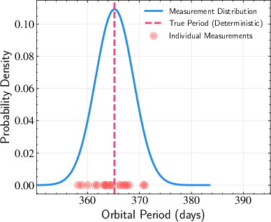
The book highlights the distinction between deterministic and random variables, noting that even deterministic quantities become random when subject to measurement uncertainty. (Figure 1)

Figure 1: Illustration of deterministic versus random variables. The dashed vertical line represents a true (deterministic) value of some quantity. The blue curve shows the probability distribution of measured values when accounting for uncertainties. Individual red dots represent specific measurements, which scatter around the true value due to various sources of uncertainty. This demonstrates how a fundamentally deterministic quantity becomes a random variable when we consider measurement or other uncertainties.

Moments of Distributions

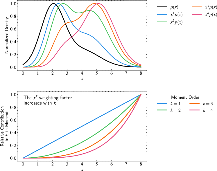
The textbook describes how different moments weight a probability distribution, with higher moments being increasingly sensitive to the tails. (Figure 2)

Figure 2: Visualization of how different moments weight a probability distribution. Top panel: The black curve shows a normalized probability distribution $p(x)$, while the colored curves show $x^k p(x)$ for different values of $k$. As $k$ increases, the peaks of $x^k p(x)$ shift toward larger values of $x$, demonstrating how higher moments become increasingly sensitive to the tails of the distribution. Bottom panel: The relative contribution of different powers of x (x^k) to each moment, showing how higher moments (k > 1) give progressively more weight to larger values. This illustrates why higher moments are particularly sensitive to extreme values in a distribution—a feature especially relevant in astronomy where rare, extreme objects often carry important physical information.

Transformation of Variables

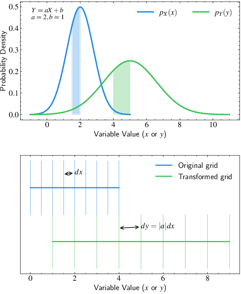
The transformation of random variables is discussed, emphasizing linear transformations and the Jacobian factor. (Figure 3)

Figure 3: Visualization of how probability distributions transform under linear transformations. Top panel: The blue curve shows the original probability distribution p_X(x) and the green curve shows the transformed distribution p_Y(y) under the linear transformation Y = 2X + 1. The shaded regions have equal areas, demonstrating probability conservation. Bottom panel: Illustration of how a uniform grid transforms under the same linear transformation. The spacing between grid lines increases by a factor of |a|=2, necessitating a corresponding decrease in probability density by a factor of 1/|a| to preserve total probability. This visualization demonstrates why the Jacobian factor |dx/dy| appears in probability transformation formulas.

Law of Total Expectation

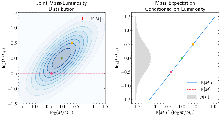
The law of total expectation is visualized using stellar mass-luminosity relationships. (Figure 4)

Figure 4: Visualization of the law of total expectation using stellar mass-luminosity relationships. Left panel: Joint distribution of stellar mass and luminosity (in solar units and log scale), shown as blue contours. The red cross marks the overall expectation $\mathbb{E}[M]$, while colored circles show conditional expectations $\mathbb{E}[M|L]$ at three different luminosities (marked by dashed lines). Right panel: The conditional distribution $p(L)$, which accounts for observational selection effects in magnitude-limited surveys.

Impact of Correlation

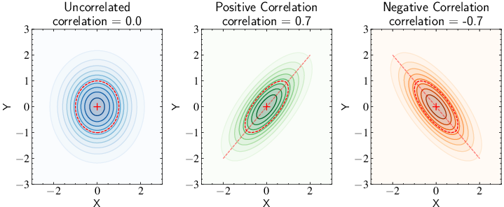
The impact of correlation on bivariate normal distributions is demonstrated. (Figure 5)

Figure 5: Visualization of how correlation shapes bivariate normal distributions. The panels show three distributions with identical marginal variances but different correlation structures. Left panel: Uncorrelated variables (rho = 0) produce circular contours, with the principal axes of the red dashed ellipse aligned with the coordinate axes. Middle panel: Positive correlation (rho = 0.7) stretches the distribution along the diagonal (red dashed line), indicating that higher values of one variable tend to occur with higher values of the other. Right panel: Negative correlation (rho = -0.7) tilts the distribution in the opposite direction, showing that high values of one variable tend to occur with low values of the other. The red dashed ellipses, representing contours of constant probability, rotate and deform based on the correlation strength, while maintaining the same total variance (area). This illustrates how correlation captures the directionality of the relationship between variables without affecting their individual scales.

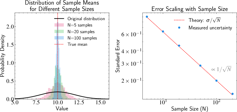
Sample Mean Uncertainty

The textbook includes an illustration of how sample mean uncertainty decreases with sample size. (Figure 6)

Figure 6: Demonstration of how sample mean uncertainty decreases with sample size. Left panel: The black curve shows the original distribution of individual measurements (with true mean shown by red dashed line). The colored histograms show the distributions of sample means for different sample sizes (N=5, 20, and 100). As N increases, the distribution of sample means becomes increasingly concentrated around the true mean, demonstrating how larger samples provide more precise estimates. Right panel: Quantitative analysis of how the standard error (uncertainty in the sample mean) scales with sample size. The red dashed line shows the theoretical prediction $\sigma/\sqrt{N}$, while blue points show the measured uncertainties from numerical simulations.

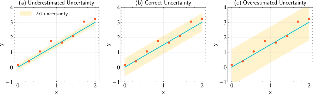
Addressing Uncertainty

Different choices of uncertainty values affect the likelihood in maximum likelihood estimation. (Figure 7)

Figure 7: Demonstration of how different choices of uncertainty values affect the likelihood in maximum likelihood estimation. Panel (a): With underestimated uncertainties (sigma = 0.1), the narrow Gaussian distributions mean data points far from the model contribute very small likelihood terms, resulting in a low total likelihood. Panel (b): When uncertainties are correctly estimated (sigma = 0.3), we achieve the maximum likelihood—this represents the optimal balance between the width of the Gaussian distributions and their heights. Panel (c): With overestimated uncertainties (sigma = 0.6), while the Gaussian distributions are wide enough to encompass most points, the height of each Gaussian (which scales as 1/\sigma) becomes smaller, resulting in smaller likelihood values overall.

Bayesian Framework

In Bayesian inference, models that maximize $p(\mathcal{D} | \boldsymbol{\theta})$ become more probable in our posterior distribution $p(\boldsymbol{\theta} | \mathcal{D})$. The textbook has a lot of visualizations to represent these concepts.

Conclusion

"Statistical Machine Learning for Astronomy" (2506.12230) serves as a comprehensive resource for astronomers seeking to understand and apply machine learning techniques within a rigorous statistical framework. Its emphasis on theory, clear explanations, and astronomical applications makes it a valuable tool for researchers navigating the complexities of modern data analysis.