Discovery of Unstable Singularities
Abstract: Whether singularities can form in fluids remains a foundational unanswered question in mathematics. This phenomenon occurs when solutions to governing equations, such as the 3D Euler equations, develop infinite gradients from smooth initial conditions. Historically, numerical approaches have primarily identified stable singularities. However, these are not expected to exist for key open problems, such as the boundary-free Euler and Navier-Stokes cases, where unstable singularities are hypothesized to play a crucial role. Here, we present the first systematic discovery of new families of unstable singularities. A stable singularity is a robust outcome, forming even if the initial state is slightly perturbed. In contrast, unstable singularities are exceptionally elusive; they require initial conditions tuned with infinite precision, being in a state of instability whereby infinitesimal perturbations immediately divert the solution from its blow-up trajectory. In particular, we present multiple new, unstable self-similar solutions for the incompressible porous media equation and the 3D Euler equation with boundary, revealing a simple empirical asymptotic formula relating the blow-up rate to the order of instability. Our approach combines curated machine learning architectures and training schemes with a high-precision Gauss-Newton optimizer, achieving accuracies that significantly surpass previous work across all discovered solutions. For specific solutions, we reach near double-float machine precision, attaining a level of accuracy constrained only by the round-off errors of the GPU hardware. This level of precision meets the requirements for rigorous mathematical validation via computer-assisted proofs. This work provides a new playbook for exploring the complex landscape of nonlinear partial differential equations (PDEs) and tackling long-standing challenges in mathematical physics.
Paper Prompts
Sign up for free to create and run prompts on this paper using GPT-5.
Top Community Prompts
Explain it Like I'm 14
Overview
This paper is about a big mystery in math and physics: can the equations that describe how fluids move suddenly “blow up,” meaning certain values (like how fast the fluid is spinning) become infinite in a finite amount of time? The authors use a mix of clever math and machine learning to discover new examples of these “blow-ups,” especially the hard-to-find kind called unstable singularities. They also reach very high accuracy, good enough to help future rigorous math proofs.
Key questions the paper asks
- Can we find unstable singularities (the most delicate, easily disturbed blow-ups) in important fluid equations?
- Can we do this reliably and with such high precision that mathematicians could later turn these discoveries into proofs?
- Is there a simple pattern that connects how “unstable” a singularity is to how fast it blows up?
How they approached the problem (in everyday language)
What is a “singularity” here?
Imagine stirring a fluid. Most of the time, things stay smooth. A singularity is like a sudden, extreme event where some quantity (for example, the steepness of a wave or how quickly the fluid spins) skyrockets to infinity in a finite time. It’s like a whirlpool that gets sharper and sharper until it becomes infinitely sharp.
Stable vs. unstable singularities
- Stable singularity: Like a ball at the bottom of a bowl. If you nudge it a bit, it rolls back and still falls into the same spot. These are easier to find with simulations.
- Unstable singularity: Like trying to balance a pencil on its tip. The tiniest breath of air will make it fall. These are very hard to find and keep track of in computations because even tiny errors push you off course.
The paper focuses on finding the unstable kind, which many believe are the ones that matter most for the hardest open problems (like the famous Navier–Stokes Millennium Prize Problem).
Self-similar coordinates: zooming in smartly
Near a singularity, things change very fast. To handle that, the authors use “self-similar coordinates.” Think of zooming in on a tornado so that, as time goes on, the picture keeps the same shape while you rescale space and time. In these coordinates, instead of simulating a wild movie, you “freeze” the picture and look for a smooth, steady shape (the “profile”) and a number that controls how fast it blows up (called the scaling rate, written as ).
- The job becomes: find the smooth profile and the right that make the transformed equations hold everywhere.
How they used machine learning (PINNs) plus a precise optimizer
- PINNs (Physics-Informed Neural Networks) are neural networks that are trained to satisfy the equation itself (not just data). You feed the network the coordinates; it outputs the solution; and the training loss tells you how badly it disobeys the physics.
- They build the network with math “hints”:
- Impose symmetries and boundary behavior.
- Transform infinite domains into manageable ones.
- Use “solution envelopes” to bake in how the solution behaves near the center and far away.
- Use math relationships to guide or even determine instead of guessing it.
- High-precision training:
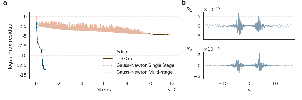
- They use a Gauss–Newton optimizer (a powerful, second-order method) instead of standard optimizers like Adam or L-BFGS. This helps reach much higher accuracy.
- They also use “multi-stage training”: train one network to get close, then train a second to fix the leftover errors (especially high-frequency wiggles).
Checking that the solutions are real and accurate
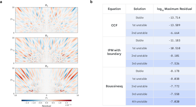
- Residual check: Plug the network’s solution back into the equations everywhere and measure the largest error (the “maximum residual”). Smaller is better.
- Stability check: Linearize the equations around the found profile and count how many directions are unstable. For the “-th unstable” solution, you should see unstable directions. This is exactly what they find.
- Precision: For some solutions (in a simpler 1D model known as CCF), they get errors as small as about , which is near the limit of standard computer number precision.
Main findings and why they matter
- They discovered several new unstable self-similar singularities in:
- The CCF model (a simplified equation related to fluid motion),
- The 2D incompressible porous media (IPM) equation,
- The 2D Boussinesq equations (with a boundary), which are closely related to the 3D Euler equations with axial symmetry and a boundary.
- They achieved very high accuracy:
- Typical errors around to for IPM and Boussinesq,
- Near machine precision (about ) for certain CCF solutions.
- This level of accuracy is a key requirement for rigorous computer-assisted proofs.
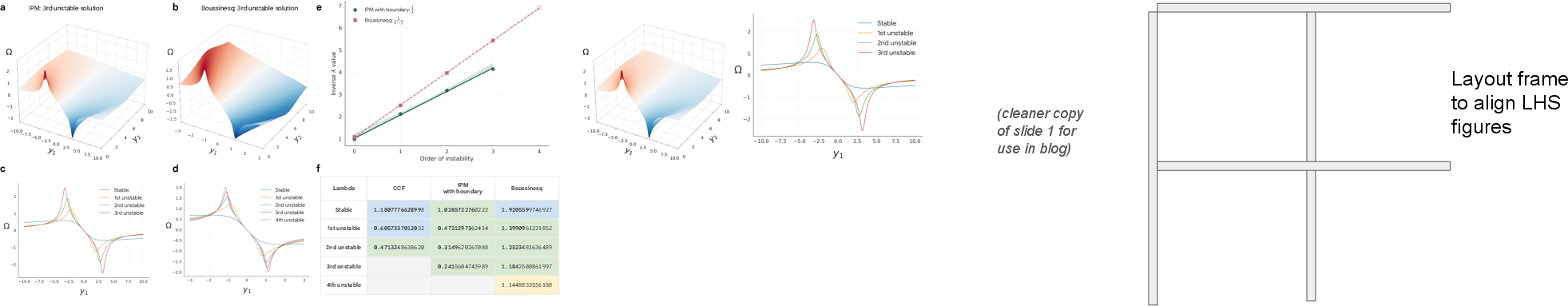
- They found a simple pattern linking instability level and blow-up speed:
- Each unstable solution has a scaling rate . Smaller means more unstable and faster blow-up.
- For Boussinesq/Euler-with-boundary and IPM, they observed an almost linear rule for how changes as the number of unstable directions grows. In short, as increases, follows a simple trend you can predict.
- They improved what we know about when dissipation still allows blow-up in the CCF model:
- They found higher-order unstable solutions and refined earlier ones, pushing the boundary (a parameter often called ) up to about $0.68$ for which blow-up is expected. This sharpens our understanding of when “smoothing effects” can and cannot stop singularities.
Why this is important:
- Unstable singularities are believed to be the kind relevant to the hardest open problems, like whether the famous Navier–Stokes equations can blow up.
- Having a reliable way to discover and verify such solutions is a significant step forward, and their extreme accuracy opens the door to formal mathematical proofs.
What this could lead to
- A new “playbook” for exploring very complex fluid equations:
- Combine math insights (symmetry, scaling, boundary behavior) with specialized machine learning and high-precision optimization.
- Better guidance for future searches:
- The simple patterns in give good starting guesses for finding even higher-order unstable solutions.
- Progress toward big open problems:
- Although the toughest case (like the 3D Euler/Navier–Stokes without boundaries) remains unsolved, this work develops the tools and strategies likely needed to tackle it.
- Stronger bridges between computation and proof:
- Solutions accurate enough for computer-assisted proofs can help turn numerical discoveries into theorems, advancing both mathematics and physics.
In short, the authors show how to reliably find the most delicate kinds of fluid “blow-ups,” do it with record-setting precision, and uncover simple rules behind them—all of which could help unlock long-standing mysteries about how fluids behave at their most extreme.
Knowledge Gaps
Knowledge gaps, limitations, and open questions
Below is a concise, actionable list of what remains missing, uncertain, or unexplored in the paper.
- Boundary-free Euler/Navier–Stokes singularities: No unstable self-similar solutions were discovered for boundary-free 3D Euler or Navier–Stokes; existence, structure, and admissible sequence in the boundary-free setting remain open.
- Rigorous validation (CAP) beyond CCF: Computer-assisted proofs are only indicated as “in preparation” for CCF; rigorous interval-arithmetic validation, enclosure of , and certified residual bounds for IPM and Boussinesq profiles are not yet provided.
- Fourth unstable Boussinesq profile unresolved: The candidate 4th unstable solution is not validated (no reliable or residual certification); a precise workflow to achieve CAP-level accuracy is missing.
- Completeness and uniqueness at fixed instability order: It is not established whether the -th order unstable singularity is unique (up to symmetries) or whether multiple discrete solutions (or continua) exist for the same instability order.
- Symmetry restrictions in discovery and stability: All solutions and linear stability analyses are performed under specific symmetry/parity and boundary conditions; symmetry-breaking modes, non-axisymmetric perturbations, and alternative boundary geometries are not analyzed.
- Linear vs nonlinear stability: Only linear spectra are computed; nonlinear (in)stability, mode coupling, and behavior along center/unstable manifolds are unquantified.
- Dynamical realization and manifolds: There is no time-dependent verification that trajectories in rescaled variables approach/repel the computed profiles; the dimension/codimension and structure of stable/unstable manifolds, and explicit construction of initial data that land on these trajectories, are not characterized.
- Empirical –instability law lacks theory: The observed linear law of inverse scaling rate vs instability order for IPM and Boussinesq is empirical; its theoretical derivation, range of validity, asymptotics as , and error quantification are open.
- No asymptotic law for CCF: Higher-order unstable CCF profiles are not available at sufficient accuracy to infer an asymptotic relationship; it remains unclear whether a similar linear trend holds.
- Fractional dissipation thresholds in CCF: Only up to the second unstable profile is used to update the critical threshold (to ); whether higher-order profiles further raise this threshold or yield the optimal bound is unknown.
- Viscous persistence: The conjecture that higher-instability Euler/Boussinesq/IPM profiles persist under viscosity (Navier–Stokes or fractional dissipation) is untested; quantitative regimes, scaling laws, and perturbative matching are not established.
- Effects of exponentially small boundary terms: For the Boussinesq/Euler analogy “up to exponentially small terms,” the impact of these corrections on high-order unstable solutions, their spectra, and is not quantified.
- Residual metric adequacy: Accuracy is reported via maximum PDE residual on a dense grid; rigorous a posteriori error estimators in continuous norms, aliasing analysis, and guarantees against grid-induced bias are missing.
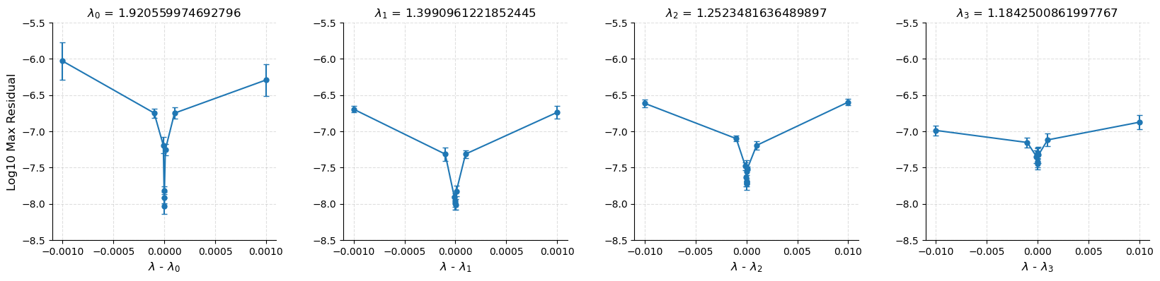
- identification and uncertainty: The selection via smoothness constraints and perturbation tests lacks rigorous uniqueness and error bars; sensitivity to the choice of solution envelope and coordinate transforms is not quantified.
- Sensitivity to architecture and training choices: The dependence of discovered solutions on PINN architecture, activation functions, solution envelopes, compactification maps, sampling strategy, and multistage training is not systematically studied.
- Scalability of optimization: The full-matrix Gauss–Newton approach depends on small networks; how to scale to higher-dimensional, less symmetric problems (e.g., full 3D Euler without boundaries) while maintaining precision remains open.
- Precision and reproducibility: Results rely on GPU double precision and report being round-off limited; reproducibility across hardware, potential benefits of arbitrary-precision arithmetic, and formal uncertainty quantification for eigenvalues//residuals are not addressed.
- Infinite-domain modeling choices: The compactification and envelope factors may bias the solution space; comparisons with alternative bases (e.g., rational spectral, conformal maps) and their effect on accuracy and discoverability are not explored.
- Time-integration verification: Stabilized time-stepping or shadowing methods to confirm self-similar attractor/repellor behavior in full PDE dynamics near the candidate profiles are not presented.
- Higher-order solutions beyond those reported: Systematic procedures and initializations to robustly discover higher-order unstable Boussinesq/IPM/CCF solutions (beyond those obtained here) are not established.
- Physical interpretability and detection: How instability order and map to observable signatures in direct numerical simulations or experiments, and how to target or detect specific unstable profiles in practice, are not specified.
- Extension to other PDEs: The approach is not tested on related equations with known or suspected unstable blow-up (e.g., SQG, vortex sheets, water waves, non-axisymmetric 3D Euler); transferability and required adaptations are unknown.
- Data/code availability for community CAP: Public release of profiles, values, training configurations, and validation grids to facilitate independent CAPs and benchmarking is not specified.
Glossary
- Admissible λ: Values of the self-similar scaling parameter that admit smooth self-similar solutions in the rescaled coordinates. Example: “By construction, finding a self-similar singularity entails the task of identifying λ values admitting smooth solutions… We say such values of λ are admissible.”
- Asymptotic formula: An expression describing limiting behavior (e.g., for large instability order) that approximates relationships among quantities. Example: “Revealing a simple empirical asymptotic formula relating the blow-up rate to the order of instability.”
- Axisymmetric: Symmetric around a central axis; here, a symmetry class of 3D Euler flows. Example: “Finite-time blow-up for the axisymmetric 3D Euler equations if one introduces a cylindrical boundary.”
- Boussinesq equations: A PDE system modeling buoyancy-driven flows in fluids (important in geophysical fluid dynamics). Example: “The Boussinesq equations… model atmospheric flows.”
- Boundary-free: A problem setup with no physical boundary, often making singularities more elusive. Example: “Boundary-free Euler and Navier-Stokes cases, where unstable singularities are hypothesized to play a crucial role.”
- B-splines: Piecewise polynomial basis functions used in numerical approximation, often on non-uniform meshes. Example: “Previous frameworks utilizing numerical tools such as B-splines on non-uniform meshes… excel at resolving stable blow-up solutions.”
- Burgers’ equation: A simplified nonlinear PDE used as a model for transport and shock formation. Example: “Illustrated in (i) with Burgers’ Equation.”
- Córdoba-Córdoba-Fontelos (CCF) equations: A 1D nonlocal transport model used as a simplified analogue for fluid singularity studies. Example: “Crucially, for specific solutions (the Córdoba-Córdoba-Fontelos (CCF) stable and 1st unstable solutions), we reach near double-float machine precision.”
- Colliding dipoles: A proposed blow-up scenario in Euler flows involving interacting vortex dipoles. Example: “Several works have considered the possibility of colliding dipoles.”
- Compactification (of infinite domains): Coordinate transformations that map an unbounded spatial domain to a bounded one to ease computation. Example: “Infinite domains… are handled using coordinate transformations that compactify the space.”
- Computer-assisted proof (CAP): A rigorous proof framework using validated numerics (e.g., interval arithmetic) to certify mathematical statements. Example: “A computer-assisted proof (CAP) via the use of interval arithmetic.”
- Continuation methods: Numerical techniques that track solutions as a parameter varies; can fail when solutions are discrete rather than forming a continuum. Example: “When those solutions are quantized… continuation methods cannot be applied.”
- Darcy’s law: A constitutive law describing flow through porous media, relating velocity to pressure gradient. Example: “The IPM equations describe density evolution driven by incompressible flows governed by Darcy’s law under gravity.”
- Defocusing Nonlinear Schrödinger (NLS) equation: A dispersive PDE where nonlinearity defocuses waves; used as an analogy for blow-up analysis. Example: “This phenomenon has been observed in… the defocusing Nonlinear Schrödinger (NLS) equation.”
- Dissipation (fractional dissipation): Regularizing effects, often modeled by fractional Laplacian operators . Example: “An important open question… is whether singularities still occur in the presence of fractional dissipation .”
- Double-floating-point machine precision: Accuracy near the limits of 64-bit floating-point arithmetic, constrained by round-off. Example: “We reach near double-float machine precision, attaining a level of accuracy constrained only by the inherent round-off errors of the GPU hardware.”
- Euler equations (3D Euler): PDEs for inviscid, incompressible fluid flow; central to singularity formation questions. Example: “Whether singularities can form in fluids… such as the 3D Euler equations.”
- Finite elements: A numerical method that approximates PDE solutions using piecewise polynomial basis on a mesh. Example: “Finite elements… excel at resolving stable blow-up solutions.”
- Finite-time blow-up: Formation of singularities (e.g., infinite gradients) in a solution within a finite time. Example: “Develop infinite gradients or velocities in finite time.”
- Gauss–Newton optimizer: A second-order optimization method for least-squares problems, leveraging curvature information. Example: “A high-precision Gauss-Newton optimizer, achieving accuracies that significantly surpass previous work.”
- Incompressible Porous Media (IPM) equation: A PDE describing density-driven flow through porous material under incompressible conditions. Example: “We present multiple new, unstable self-similar solutions for the incompressible porous media equation.”
- Instability order: The number of unstable directions (modes) of a solution; higher order indicates greater instability. Example: “Inverse scaling rate versus the instability order… reveals a linear trend.”
- Interval arithmetic: Numerical computations with intervals to rigorously bound errors and certify results. Example: “A computer-assisted proof (CAP) via the use of interval arithmetic.”
- Linearisation: Approximating a nonlinear PDE around a solution by its linear counterpart to analyze stability (spectrum, modes). Example: “We analyze the spectrum of the linearisation of the governing equations around the candidate solution.”
- Maximum residual: The largest absolute PDE violation when substituting a candidate solution into the equations over the domain. Example: “We quantify the accuracy… using the maximum residual.”
- Multi-stage training: A training scheme where successive networks correct residual errors to reach higher precision. Example: “Multi-stage training is able to further improve the results by five orders of magnitude.”
- Navier–Stokes equations: Viscous counterparts to Euler equations; central to the Millennium Prize Problem. Example: “The 3D Navier-Stokes equations… represent perhaps the most famous case.”
- Nonlocal drift: Velocity field depending nonlocally on the transported quantity, typical in active scalar and CCF-type models. Example: “A transport equation with nonlocal drift.”
- Physics-Informed Neural Networks (PINNs): Neural networks trained to satisfy PDEs via loss terms encoding physics and boundary conditions. Example: “We use a Physics-informed Neural Network (PINN) with a Gauss-Newton optimiser…”
- Round-off errors: Numerical errors due to finite-precision arithmetic in hardware. Example: “Constrained only by the inherent round-off errors of the GPU hardware.”
- Scaling parameter λ: The self-similar rate controlling space-time rescaling and blow-up structure. Example: “A self-similar scaling rate λ… finding the right scaling rate λ.”
- Self-similar coordinates: Rescaled space-time variables centered on blow-up to convert time evolution into a stationary profile problem. Example: “These coordinates rescale space and time around the point of blow-up… transforming the problem… into finding a stationary, smooth self-similar profile.”
- Self-similar profile: The stationary solution in self-similar coordinates representing the blow-up shape. Example: “Finding a stationary, smooth self-similar profile.”
- Spectral methods: Numerical techniques using global basis functions (e.g., Fourier/Chebyshev) to solve PDEs. Example: “Spectral methods… excel at resolving stable blow-up solutions.”
- Stability analysis: Assessing whether perturbations grow or decay by studying linearised dynamics around a solution. Example: “We conduct a stability analysis by linearizing the governing equations around the solution.”
- Stable singularity: A singularity that forms robustly under small perturbations of initial data. Example: “A stable singularity is a robust outcome, forming even if the initial state is slightly perturbed.”
- Unstable manifold: The set of perturbation directions along which solutions diverge from a trajectory (e.g., blow-up path). Example: “Overcome the exponential instabilities arising from being on the unstable manifold.”
- Unstable modes: Eigen-directions of the linearised operator with positive growth, indicating instability of the solution. Example: “We find n unstable modes that respect the same symmetry assumptions as the solution.”
- Unstable singularity: A singularity requiring infinitely precise initial conditions; small perturbations prevent blow-up along that trajectory. Example: “Unstable singularities… require initial conditions tuned with infinite precision… infinitesimal perturbations immediately divert the solution from its blow-up trajectory.”
- Viscous terms: Additions (e.g., diffusion) to a PDE that introduce viscosity and can stabilize or regularize solutions. Example: “Hou added viscous terms to stabilize the blow-up.”
- Vorticity: The curl of the velocity field, measuring local rotation in fluid flow. Example: “Spatial profile of the vorticity Ω for the third unstable solutions… near the origin.”
Collections
Sign up for free to add this paper to one or more collections.

