A Time Series Model for Three Asset Classes used in Financial Simulator (2508.06010v1)
Abstract: We create a dynamic stochastic general equilibrium model for annual returns of three asset classes: the USA Standard & Poor (S&P) stock index, the international stock index, and the USA Bank of America investment-grade corporate bond index. Using this, we made an online financial app simulating wealth process. This includes options for regular withdrawals and contributions. Four factors are: S&P volatility and earnings, corporate BAA rate, and long-short Treasury bond spread. Our valuation measure is an improvement of Shiller's cyclically adjusted price-earnings ratio. We use classic linear regression models, and make residuals white noise by dividing by annual volatility. We use multivariate kernel density estimation for residuals. We state and prove long-term stability results.
Paper Prompts
Sign up for free to create and run prompts on this paper using GPT-5.
Top Community Prompts
Explain it Like I'm 14
What this paper is about
This paper builds a realistic, math-based model to predict how three types of investments might behave each year:
- USA stocks (like the S&P 500 index)
- International stocks (non‑US stock markets)
- USA corporate bonds (investment‑grade bonds)
The authors use this model to power a free online financial simulator that helps people explore saving and retirement, including regular deposits or withdrawals. They also introduce a new way to judge whether the stock market is “expensive” or “fairly priced,” improving on a popular measure called CAPE.
The big questions the paper asks
- Is the stock market really overvalued today, even though CAPE is high?
- Can we build a simple, reliable model that uses a few key signals to forecast returns for stocks and bonds?
- Do returns behave more “normally” if we first account for how bumpy the market is (its volatility)?
- Can we prove the model is stable in the long run, so the simulator doesn’t drift into unrealistic outcomes?
How the model works (in everyday language)
Key ideas in plain words
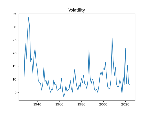
- Volatility: Think of the stock market like a road. Some years it’s smooth; other years it’s full of bumps. Volatility measures how bumpy the ride is.
- Earnings: Companies make profits (earnings). Over time, earnings grow (or shrink). Earnings are a “fundamental” that helps value stocks.
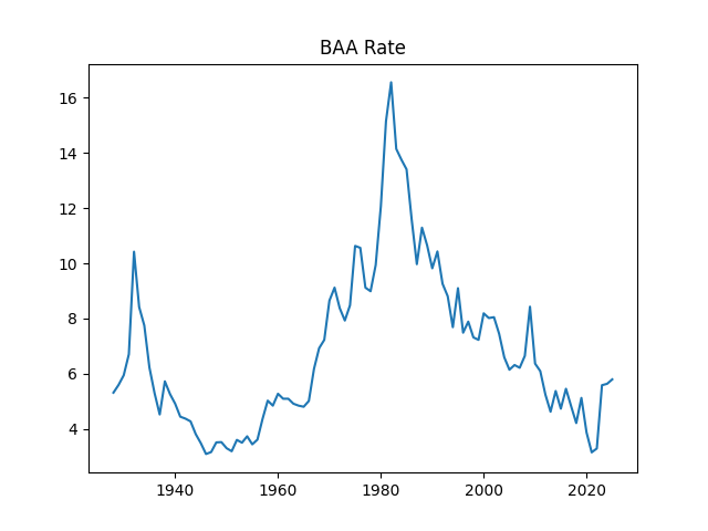
- Interest rates: Bonds pay interest. Corporate bonds (rated BAA) are like loans to companies. The “rate” is the cost of borrowing. Higher rates can make bonds more attractive than stocks.
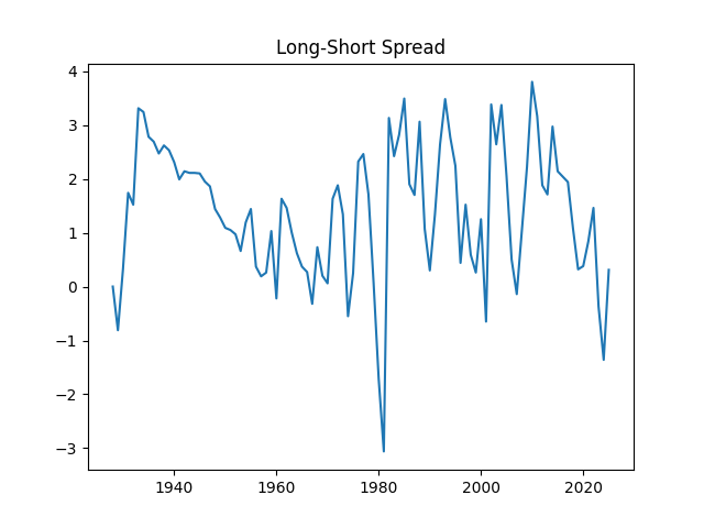
- Term spread: The difference between long‑term and short‑term government interest rates. When long‑term rates drop below short‑term rates (an “inverted yield curve”), a recession often follows.
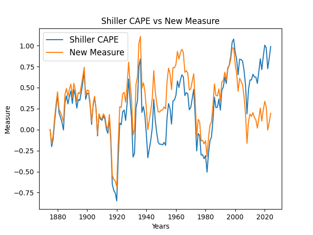
The improved valuation measure (fixing CAPE)
CAPE compares stock prices to average earnings over 10 years. It worked well for over a century, but in recent decades companies have paid fewer dividends and done more stock buybacks. That makes prices rise without increasing dividends, which can make CAPE look “too high” even when the market isn’t in a bubble.
So the authors created a new valuation measure:
- Add up total stock returns over time (including dividends).
- Subtract how fast earnings have grown.
- Remove a steady long‑term trend (about 4–5% per year), because stock returns historically outpace earnings by that amount.
- What’s left tends to move back toward normal over time (this behavior is called “mean reversion”). This new measure matched CAPE before 2000, but after that it stayed near normal while CAPE shot up—suggesting the market is not wildly overpriced today.
Making messy data easier to model
The authors discovered something very useful: if you divide yearly stock returns and yearly earnings growth by the market’s yearly volatility, the results behave much more like pure randomness (“white noise”), which is easier and safer to model. In simple terms, once you account for how bumpy the year was, what’s left looks like fair‑game luck.
They then:
- Modeled volatility itself using an “AR(1)” model, which means each year’s volatility partly depends on last year’s (like a rubber band that snaps back toward normal).
- Modeled the BAA corporate bond rate in a similar way (with some signs it behaves close to a random walk).
- Modeled the term spread (long‑minus‑short interest rates) as mean‑reverting.
- Built regression equations for returns of US stocks, international stocks, and corporate bonds using these factors.
A note on “white noise,” “Gaussian,” and “kernel density”
- White noise: Think of rolling a fair die or flipping a coin—no patterns.
- Gaussian: The common bell‑curve shape (normal distribution). Some parts of the model fit this shape; others don’t.
- Kernel density estimation: A flexible way to “draw the shape” of randomness without forcing it into a bell curve.
Where the data comes from
They used well‑known sources: Robert Shiller’s data library (Yale), Federal Reserve (FRED), Yahoo Finance, and MSCI indexes. They focused on:
- End‑of‑year S&P 500 levels (more realistic for investors than monthly averages)
- Annual returns (including dividends), earnings, and realized volatility
- Corporate bond rates and Treasury yields (to build the term spread)
What they found and why it matters
1) The new valuation measure fits reality better than CAPE today
- It agrees with CAPE for major past bubbles (1920s, 1960s, 1990s).
- Since 2000, CAPE stays high but the new measure stays near normal—supporting the idea that today’s market isn’t wildly overpriced once you account for buybacks and payout changes.
2) Volatility is a “universal” helper
- Dividing stock returns and earnings growth by volatility makes them behave like random noise.
- That makes the model cleaner and predictions more trustworthy.
3) US stock returns depend on several factors, all with significant effects
In their regression for US stocks, these mattered:
- Valuation (their new measure): When the market gets “too pricey,” future returns tend to be lower.
- Interest rate changes: Bigger rate increases tend to hurt stock returns.
- Term spread: A tighter or inverted spread often signals trouble ahead for stocks.
- Volatility: It affects the scale of returns and is included directly in the formula.
This regression explained about half of the year‑to‑year variation (R2 ≈ 53%), which is strong for finance.
4) International stocks also respond to US conditions, but less strongly
- US volatility and US rate changes matter.
- The valuation signal is weaker for non‑US markets.
- Overall fit is still decent (R2 ≈ 41%).
5) Corporate bond returns behave as expected
- They depend on the current rate and how much rates change.
- The model includes “duration” (how sensitive bond prices are to rate moves), and it estimates about 5.5 years—reasonable for investment‑grade bonds.
6) The model is stable long‑term
- The authors prove the system settles into a steady pattern over time (stationarity).
- That’s crucial for a simulator: you don’t want outputs that spiral unrealistically.
What this means for you and the world
- Better planning tools: The public web app lets people test saving, investing, and withdrawing (like the famous “4% rule” for retirement) under a realistic model. It includes US stocks, international stocks, and bonds, plus real‑world features like contributions and withdrawals.
- Smarter valuation: Investors and students can learn why CAPE might be misleading today and how an improved measure gives clearer signals.
- Simpler modeling: Using volatility to “normalize” returns and earnings growth makes financial modeling safer and more effective.
- Policy and education: Understanding the term spread and corporate rates helps explain why markets move around recessions and interest rate changes.
Where to try it and what’s under the hood
- Simulator: asarantsev.pythonanywhere.com
- Code and data: GitHub repository “asarantsev/sim”
- Tech stack: Python (Flask for the website), plain HTML, with statistical fitting and tests (including Monte Carlo simulations and normality checks).
Key terms in one‑liners
- Volatility: How wild the market’s ups and downs are in a year.
- Earnings growth: How fast company profits are rising.
- CAPE: A long‑term price‑to‑earnings ratio that used to be a good bubble detector.
- New valuation measure: Cumulative returns minus cumulative earnings growth, adjusted for a 4–5% long‑term trend; it mean‑reverts.
- AR(1): A model where this year partially depends on last year.
- Term spread: Long‑term rate minus short‑term rate; negative often warns of recession.
- White noise: No pattern—just randomness.
- Stationarity: A system that settles into a stable pattern over time.
Final takeaway
By carefully cleaning the data (especially using volatility) and tying together a few powerful signals—valuation, rates, spreads, and earnings—the authors built a stable, evidence‑based model of stock and bond returns. It explains history better than CAPE in modern times and powers a practical, free simulator for planning your financial future.
Collections
Sign up for free to add this paper to one or more collections.