- The paper demonstrates that decoder layer transformations are nearly linear (e.g., with a 0.99 score), challenging traditional views on transformer complexity.
- It employs a comprehensive empirical methodology using Procrustes similarity and cosine regularization to manage and analyze linearity dynamics.
- The study introduces layer pruning and linear approximations, showing that reducing model complexity can maintain performance on benchmarks like SuperGLUE.
Overview
"Your Transformer is Secretly Linear" (2405.12250) presents a comprehensive investigation into the latent linear structure of transformer decoders, including widely used models such as GPT, LLaMA, OPT, and BLOOM. Through detailed empirical analysis and novel regularization strategies, the authors demonstrate that transformations between the contextualized embeddings across sequential decoder layers are almost perfectly linear—contradicting prevailing assumptions about the functional complexity of these architectures. Multiple interventions, including regularization and layer pruning, leverage these findings to enhance model efficiency while preserving or improving performance.
Empirical Evidence for Layerwise Linearity
The authors provide an extensive quantitative analysis, using a generalized Procrustes similarity metric, to measure linearity between the embedding representations of successive transformer decoder layers. They report near-unity linearity scores (e.g., 0.99), indicating that layerwise transformations closely resemble linear maps. This observation is robust across multiple open-source transformer models and persists through significant portions of pretraining.
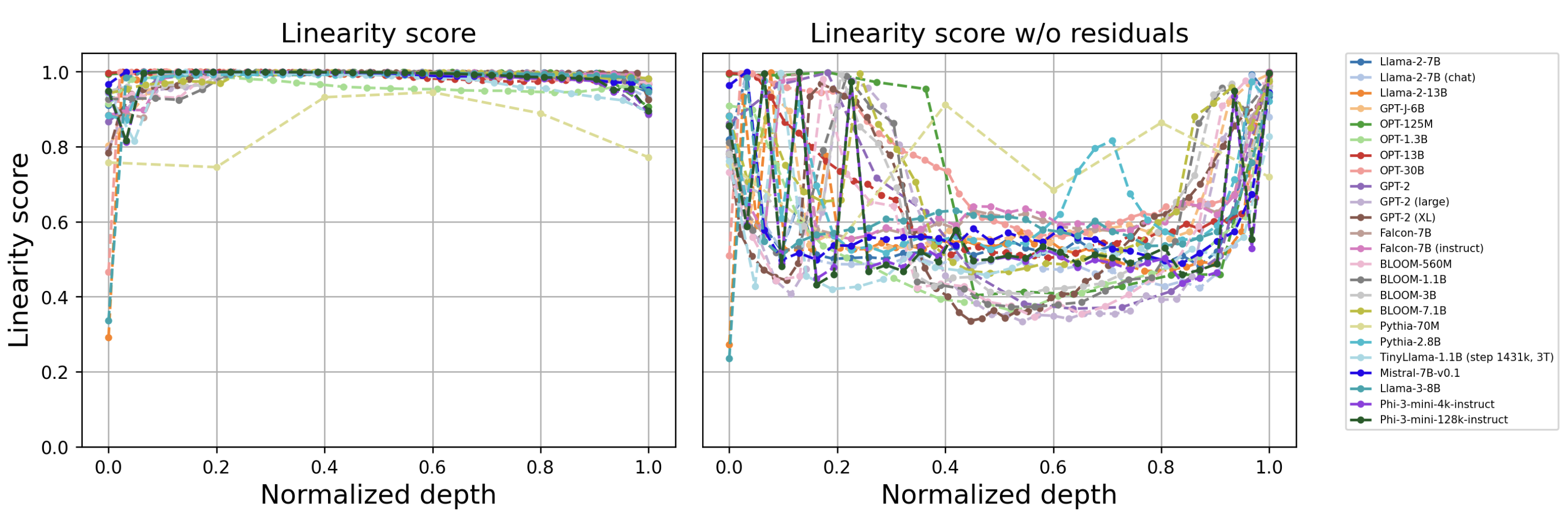
Figure 1: Linearity profiles for different open source models. Normalized depth represents layer position as a fraction of maximum model depth.
Further analysis reveals that, although the main processing stream (including residual pathways) is highly linear, removal of the residual component leads to a significant reduction in measured linearity, confirming that the low norm of each block’s contribution is pivotal. The close alignment between block output norms and the evolution of the residual stream is also visualized.
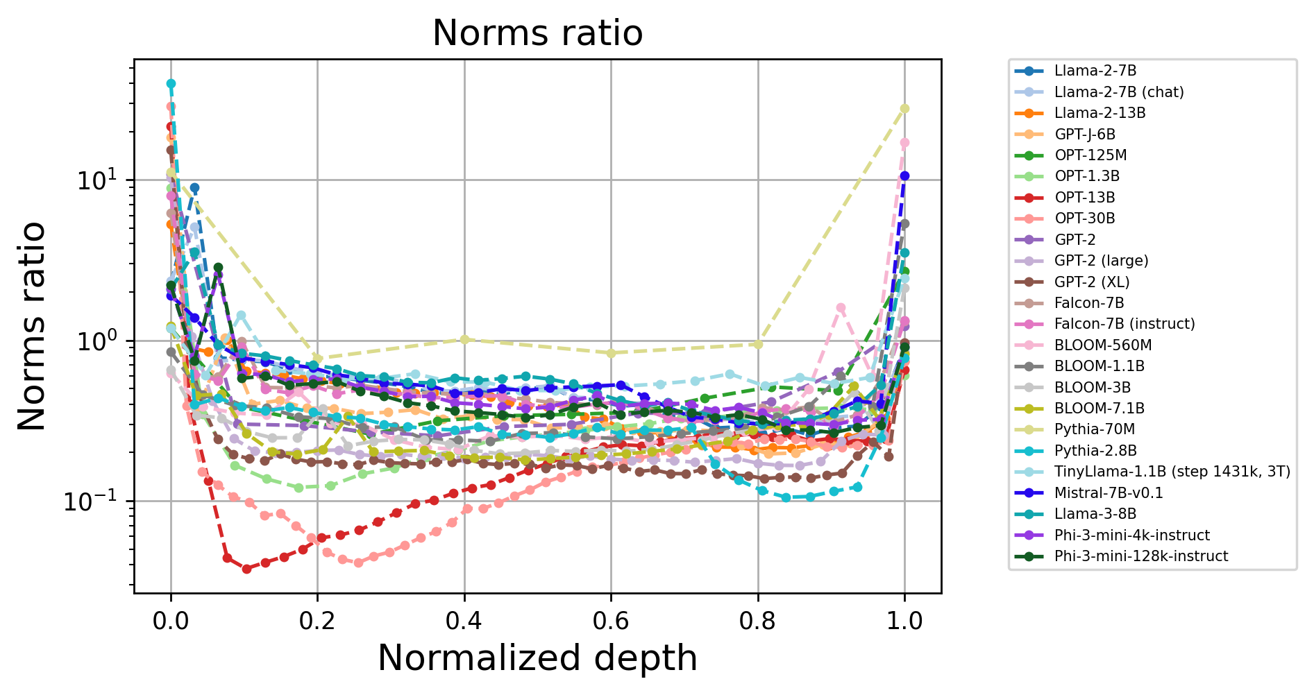
Figure 2: The output norm of each transformer block is consistently low relative to the growing norm of the residual stream, explaining high overall linearity.
Linearity Dynamics: Pretraining and Fine-Tuning
Systematic experiments across checkpoints show a monotonic decrease in overall layerwise linearity during pretraining. However, an inverse effect is observed during task-specific fine-tuning (e.g., SuperGLUE, reward modeling), where linearity increases, suggesting adaptation towards more linear representations under strong supervision.
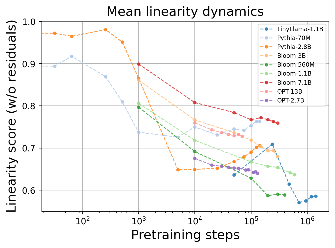
Figure 3: Average linearity score across layers declines over pretraining steps, reflecting increasing nonlinearity with model convergence.
This divergence has notable implications for regularization and transfer learning. Fine-tuned models become more linear, which may affect their ability to generalize beyond the fine-tuned distribution.
Regularization to Modulate Linearity
The paper introduces layerwise regularization strategies—specifically, mean squared error (MSE) and cosine similarity loss terms—applied to consecutive layer embeddings to control or reduce linearity. The cosine similarity regularization is particularly effective, resulting in reduced linearity as measured by the proposed score, and yielding improved performance on both TinyStories and SuperGLUE benchmarks.
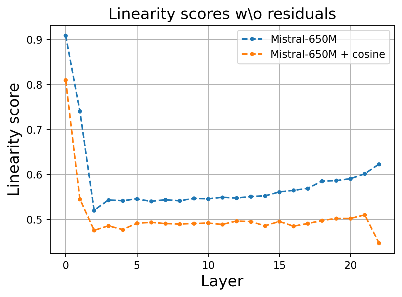
Figure 4: Cosine regularization during pretraining demonstrably reduces linearity scores in every layer.
Linear probing analysis substantiates that these regularization techniques increase the expressiveness of intermediate representations. Embeddings from regularized, less-linear models lead to improved downstream performance.
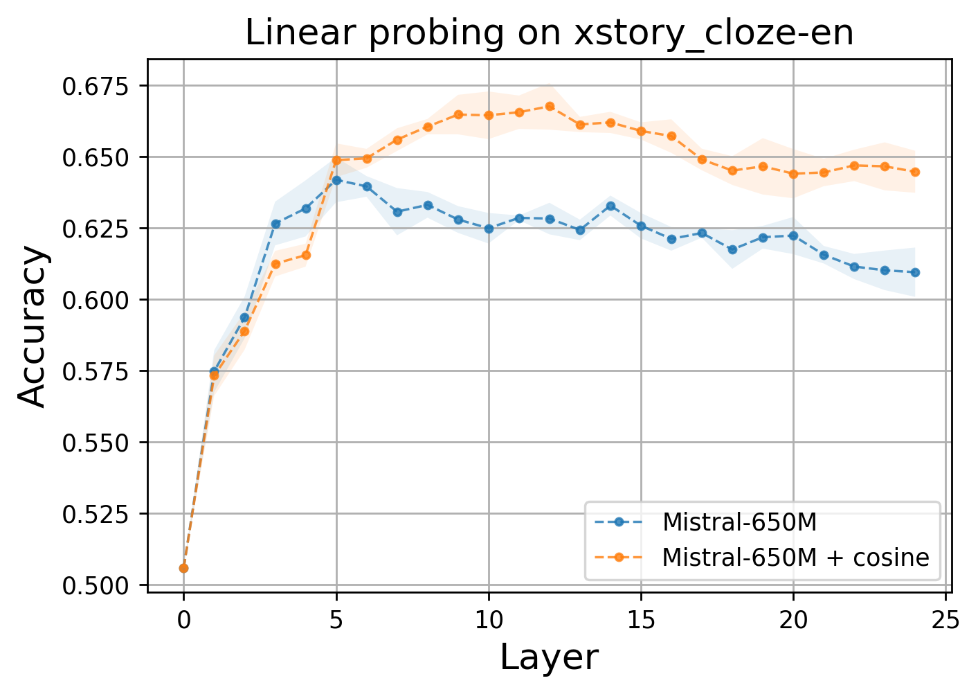
Figure 5: Linear probing accuracy on xstorycloze-en from SuperGLUE reveals superior expressiveness in regularized layers.
Interestingly, the model compensates for the increased similarity induced by the cosine regularization by amplifying non-linear effects in the residual stream, as revealed by error analyses.
Linearity-Driven Pruning and Distillation
An immediate implication of these findings is model compression. The authors exploit the fact that the most linear layers can be pruned or replaced with their best-fit linear approximation (again via Procrustes analysis), resulting in minimal degradation in perplexity or downstream accuracy. A layerwise distillation loss further aligns the compressed model’s embeddings to those of the teacher, mitigating information loss.
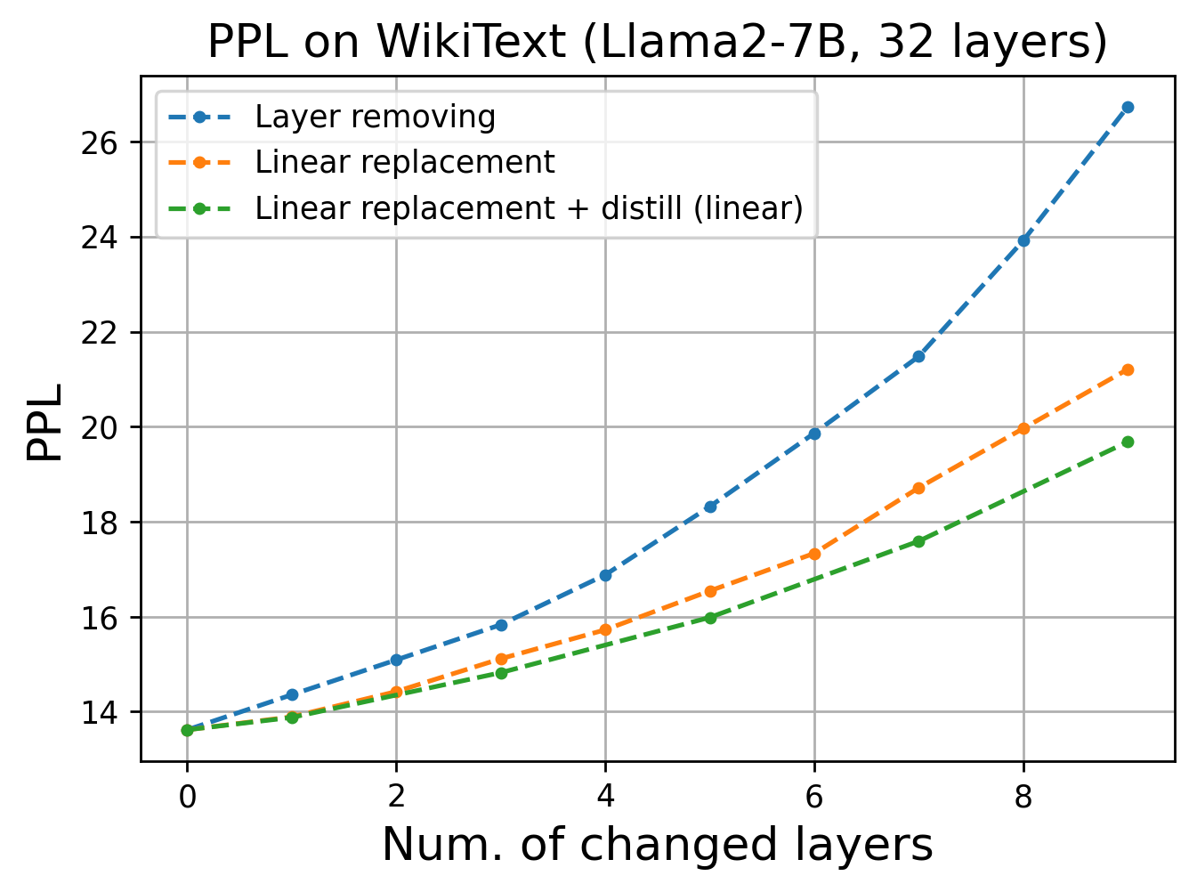
Figure 6: Perplexity comparison on WikiText shows that models with pruned layers replaced by linear projections and fine-tuned with distillation lose only marginal performance.
Additionally, the approach generalizes to large-scale models and is validated on standard benchmarks, including WikiText and ARC-Easy tasks.
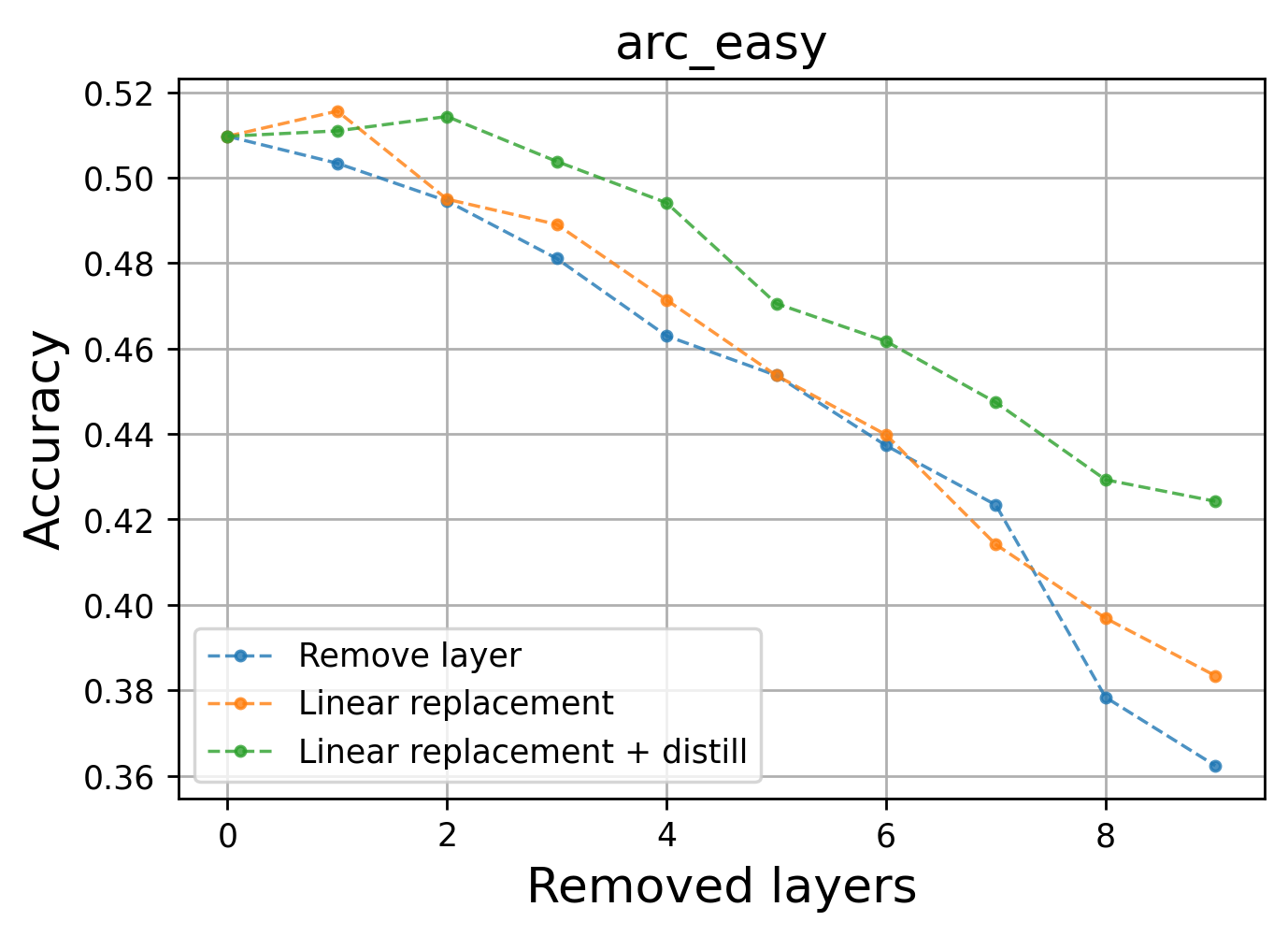
Figure 7: ARC-easy performance with layer pruning validates that highly linear layers can be pruned with little effect on task accuracy.
Finally, detailed residual error distributions reveal non-uniform, heavy-tailed components in only a few layers, supporting the hypothesis that most layers behave linearly except for rare events of high non-linearity.
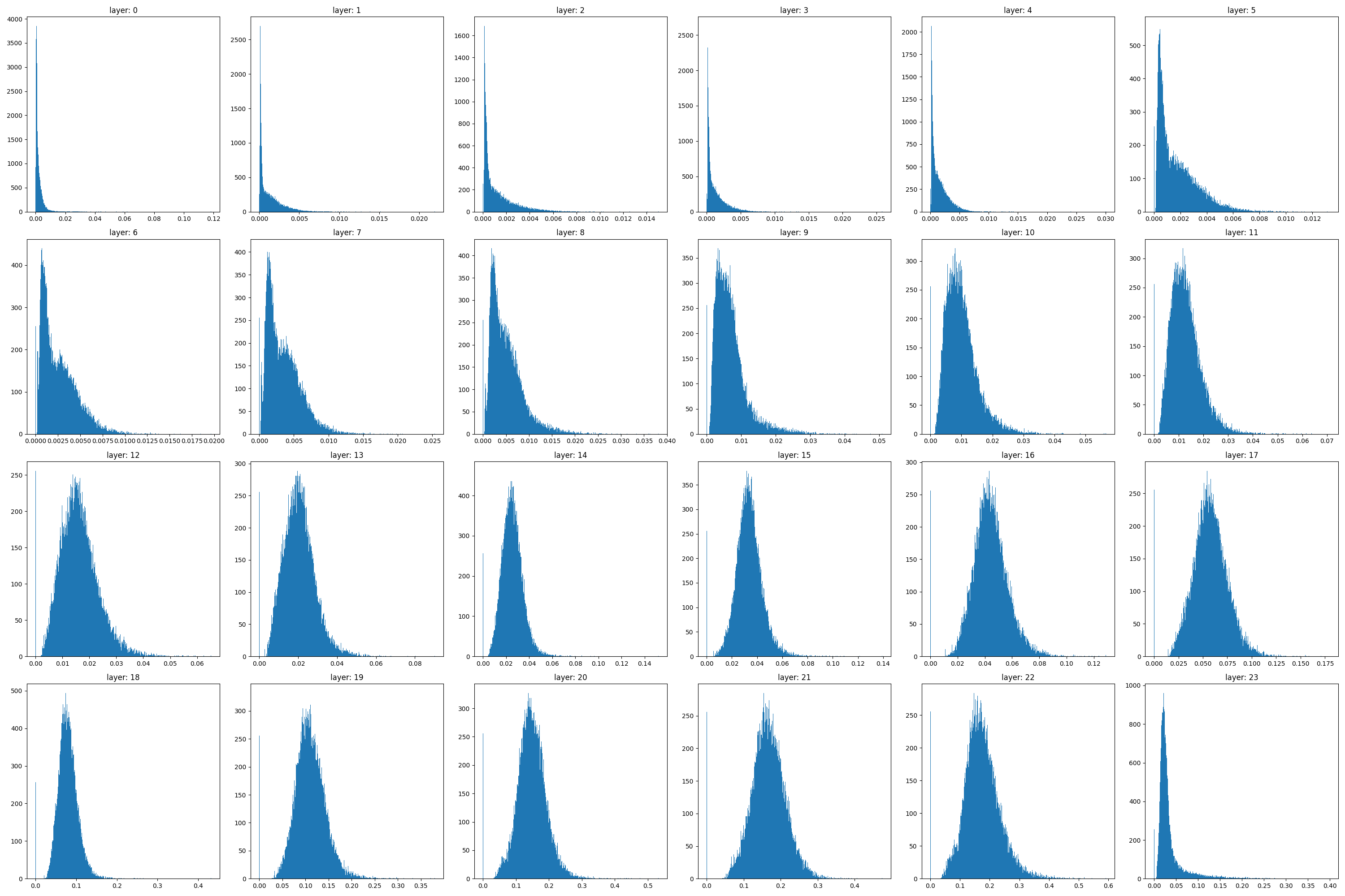
Figure 8: L2 error distribution of linear approximation in OPT-1.3B layers demonstrates high linearity interspersed with occasional large deviations.
Theoretical and Practical Implications
The near-perfect linearity of layerwise embedding transformations in transformer decoders fundamentally challenges assumptions about their internal complexity. This not only streamlines the analysis of representational dynamics but also suggests that significant portions of deep transformer architectures may be unnecessary for inference and can be replaced with linear mappings without loss of fidelity.
From a theoretical perspective, the combination of predominantly linear transformations with rare, high-nonlinearity events aligns with recent studies on neural superposition and feature triggering, indicating that complex behaviors may be encoded sporadically and sparsely in otherwise linear systems. This insight provides a new framework for understanding expressivity and capacity trade-offs in sequence models.
On the practical side, the results unlock new directions for efficient model design—layerwise pruning and linear approximations tailored via regularization produce models of lower memory and compute cost, which is valuable for deployment in resource-constrained environments. The regularization findings also raise questions about the optimality of highly linear representations for transfer and robustness.
Conclusion
This work provides a systematic dissection of transformer decoder architectures, revealing that their layerwise operations are substantially linear and can be regularized or pruned accordingly with minimal effect on global performance. These findings prompt a reevaluation of the architectural complexity needed for high-performance NLP and propose concrete strategies for compression and regularization. Future research directions include extending these analyses to encoder and encoder-decoder models, further exploring the role of rare nonlinearities, and the development of theoretical frameworks based on the observed linearity-nonlinearity dichotomy.