- The paper introduces a graph wavelet-based convolutional framework that decouples feature transformation from graph convolution to significantly reduce parameter complexity.
- It employs Chebyshev polynomial approximations to compute sparse and localized wavelet transforms, achieving high efficiency and interpretability on standard benchmarks.
- Experiments on Cora, Citeseer, and Pubmed validate that GWNN outperforms traditional spectral and spatial models in semi-supervised node classification.
Introduction
The "Graph Wavelet Neural Network" (GWNN) (1904.07785) proposes a spectral graph convolutional framework leveraging graph wavelet transforms rather than the conventional graph Fourier approaches. This work directly addresses the computational inefficiencies, lack of locality, and interpretability limitations inherent in previous spectral graph convolutional neural networks. The approach also introduces a principled decoupling of feature transformation and graph convolution, yielding significant reductions in parameter complexity, making the technique amenable to semi-supervised node classification scenarios with limited labels.
From Spectral to Wavelet-Based Graph Convolutions
Graph convolutional methods bifurcate into spatial and spectral domains. Spectral techniques define convolution in the spectral domain, relying on the eigen-decomposition of the Laplacian matrix, thereby entailing O(n3) cost and generating dense transformation matrices. Polynomial-based approximations such as ChebyNet [defferrard2016convolutional] improve efficiency but restrict flexibility and localizability. The central claim of the paper is that graph wavelet bases offer a superior solution:
- Efficient and Localized Basis: Wavelet bases can be computed via Chebyshev polynomial approximations without full eigendecomposition, providing O(m∣E∣) complexity (where m is the Chebyshev order and ∣E∣ the edge count).
- Sparsity: For real-world sparse graphs, the wavelet transform matrices possess high sparsity, drastically reducing computation relative to Fourier-based methods.
- Locality: Graph wavelets exhibit strong localization in the vertex domain, fundamentally enhancing both the theoretical interpretability and practical expressiveness of convolutions.
These properties are further illustrated by the structure of wavelets at different scales, where the scaling parameter s flexibly tunes the locality of the receptive field in a continuous, not discrete, manner.
GWNN Architecture and Parameter Decoupling
GWNN layers adopt a generalized spectral-wavelet convolutional operator. Each layer is structured as:
- Feature Transformation: Linear transformation of the per-node features.
- Graph Convolution: Application of a learnable diagonal spectral filter in wavelet space, transformed back into the vertex domain via sparse wavelet matrices.
By dissociating feature transformation from graph convolution, the model reduces the parameter complexity from O(npq) (where n is the number of nodes, p the input feature dimension, and q the output feature dimension) to O(n+pq), a crucial advantage under semi-supervised regimes with limited labeled data.
Experimental Analysis
GWNN is evaluated on standard benchmarks (Cora, Citeseer, and Pubmed) for semi-supervised node classification. The experimental setup follows established practice, with only 20 labeled nodes per class used for training. GWNN is compared against a suite of spectral (Spectral CNN, GCN, ChebyNet) and spatial (MoNet) baselines.
GWNN achieves superior accuracy across all testbeds. Notably:
- On Cora, GWNN attains 82.8% accuracy, representing an absolute gain of approximately 10% over Spectral CNN and a 1.1% improvement over GCN.
- On Citeseer and Pubmed, GWNN delivers 71.7% and 79.1% accuracy, also exceeding prior state-of-the-art spectral and spatial models.
The improvement is robust across datasets with varying sizes, feature dimensions, and label rates.
Hyperparameter Sensitivity
The model's performance is modulated by the wavelet scaling parameter s and the threshold t for wavelet matrix sparsification. As demonstrated empirically, moderate values of s optimize locality and classification accuracy, while the threshold t primarily affects computational efficiency, not prediction performance.
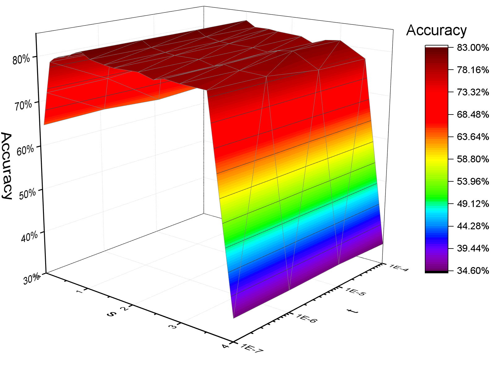
Figure 2: Influence of the scaling parameter s and the sparsification threshold t on classification accuracy for the Cora dataset.
Analysis of Sparsity and Interpretability
GWNN's wavelet transforms exhibit a density as low as 2.8% on Cora, in contrast to 99.1% for the Fourier basis. This extreme sparsity translates both to accelerated computation and to improved interpretability—projected signal patterns in the wavelet domain reveal which nodes and features interact, and the interpretability experiments underscore the semantic coherence of these interactions.
Theoretical and Practical Implications
The main theoretical implication is that computationally scalable, highly local, and interpretable spectral graph convolutions can be constructed by replacing the Fourier basis with wavelet bases obtained via Chebyshev polynomials. This approach resolves fundamental challenges in spectral GCNs related to nonlocality, computational tractability, and lack of sparsity. The explicit parameter decoupling aligns with recent deep learning trends optimizing for sample efficiency in label-sparse regimes.
Practically, GWNN's properties make it suitable for application to large-scale, sparse graphs found in citation, social, and biological networks. The approach should generalize to other graph representation tasks, including but not restricted to node clustering, link prediction, and community detection. Future work may address the method's scalability on extremely large graphs by selective wavelet basis construction and further sparsification techniques.
Conclusion
GWNN offers an efficient, interpretable, and accurate framework for spectral graph convolution via the adoption of localized wavelet transforms. This substitution brings major benefits in computational complexity, model sparsity, and interpretability, evidenced by empirical gains on standard benchmarks. By decoupling feature transformation from graph convolution, GWNN sets a paradigm for lean spectral models tailored to semi-supervised and label-limited contexts. The theoretical underpinnings and practicalities highlighted in this framework are likely to influence future graph neural network research, especially in contexts where interpretability and computational cost are primary concerns.

