Attention Is All You Need
Abstract: The dominant sequence transduction models are based on complex recurrent or convolutional neural networks in an encoder-decoder configuration. The best performing models also connect the encoder and decoder through an attention mechanism. We propose a new simple network architecture, the Transformer, based solely on attention mechanisms, dispensing with recurrence and convolutions entirely. Experiments on two machine translation tasks show these models to be superior in quality while being more parallelizable and requiring significantly less time to train. Our model achieves 28.4 BLEU on the WMT 2014 English-to-German translation task, improving over the existing best results, including ensembles by over 2 BLEU. On the WMT 2014 English-to-French translation task, our model establishes a new single-model state-of-the-art BLEU score of 41.8 after training for 3.5 days on eight GPUs, a small fraction of the training costs of the best models from the literature. We show that the Transformer generalizes well to other tasks by applying it successfully to English constituency parsing both with large and limited training data.
- Layer normalization. arXiv preprint arXiv:1607.06450, 2016.
- Neural machine translation by jointly learning to align and translate. CoRR, abs/1409.0473, 2014.
- Massive exploration of neural machine translation architectures. CoRR, abs/1703.03906, 2017.
- Long short-term memory-networks for machine reading. arXiv preprint arXiv:1601.06733, 2016.
- Learning phrase representations using rnn encoder-decoder for statistical machine translation. CoRR, abs/1406.1078, 2014.
- Francois Chollet. Xception: Deep learning with depthwise separable convolutions. arXiv preprint arXiv:1610.02357, 2016.
- Empirical evaluation of gated recurrent neural networks on sequence modeling. CoRR, abs/1412.3555, 2014.
- Recurrent neural network grammars. In Proc. of NAACL, 2016.
- Convolutional sequence to sequence learning. arXiv preprint arXiv:1705.03122v2, 2017.
- Alex Graves. Generating sequences with recurrent neural networks. arXiv preprint arXiv:1308.0850, 2013.
- Deep residual learning for image recognition. In Proceedings of the IEEE Conference on Computer Vision and Pattern Recognition, pages 770–778, 2016.
- Gradient flow in recurrent nets: the difficulty of learning long-term dependencies, 2001.
- Long short-term memory. Neural computation, 9(8):1735–1780, 1997.
- Self-training PCFG grammars with latent annotations across languages. In Proceedings of the 2009 Conference on Empirical Methods in Natural Language Processing, pages 832–841. ACL, August 2009.
- Exploring the limits of language modeling. arXiv preprint arXiv:1602.02410, 2016.
- Can active memory replace attention? In Advances in Neural Information Processing Systems, (NIPS), 2016.
- Neural GPUs learn algorithms. In International Conference on Learning Representations (ICLR), 2016.
- Neural machine translation in linear time. arXiv preprint arXiv:1610.10099v2, 2017.
- Structured attention networks. In International Conference on Learning Representations, 2017.
- Adam: A method for stochastic optimization. In ICLR, 2015.
- Factorization tricks for LSTM networks. arXiv preprint arXiv:1703.10722, 2017.
- A structured self-attentive sentence embedding. arXiv preprint arXiv:1703.03130, 2017.
- Multi-task sequence to sequence learning. arXiv preprint arXiv:1511.06114, 2015.
- Effective approaches to attention-based neural machine translation. arXiv preprint arXiv:1508.04025, 2015.
- Building a large annotated corpus of english: The penn treebank. Computational linguistics, 19(2):313–330, 1993.
- Effective self-training for parsing. In Proceedings of the Human Language Technology Conference of the NAACL, Main Conference, pages 152–159. ACL, June 2006.
- A decomposable attention model. In Empirical Methods in Natural Language Processing, 2016.
- A deep reinforced model for abstractive summarization. arXiv preprint arXiv:1705.04304, 2017.
- Learning accurate, compact, and interpretable tree annotation. In Proceedings of the 21st International Conference on Computational Linguistics and 44th Annual Meeting of the ACL, pages 433–440. ACL, July 2006.
- Using the output embedding to improve language models. arXiv preprint arXiv:1608.05859, 2016.
- Neural machine translation of rare words with subword units. arXiv preprint arXiv:1508.07909, 2015.
- Outrageously large neural networks: The sparsely-gated mixture-of-experts layer. arXiv preprint arXiv:1701.06538, 2017.
- Dropout: a simple way to prevent neural networks from overfitting. Journal of Machine Learning Research, 15(1):1929–1958, 2014.
- End-to-end memory networks. In C. Cortes, N. D. Lawrence, D. D. Lee, M. Sugiyama, and R. Garnett, editors, Advances in Neural Information Processing Systems 28, pages 2440–2448. Curran Associates, Inc., 2015.
- Sequence to sequence learning with neural networks. In Advances in Neural Information Processing Systems, pages 3104–3112, 2014.
- Rethinking the inception architecture for computer vision. CoRR, abs/1512.00567, 2015.
- Grammar as a foreign language. In Advances in Neural Information Processing Systems, 2015.
- Google’s neural machine translation system: Bridging the gap between human and machine translation. arXiv preprint arXiv:1609.08144, 2016.
- Deep recurrent models with fast-forward connections for neural machine translation. CoRR, abs/1606.04199, 2016.
- Fast and accurate shift-reduce constituent parsing. In Proceedings of the 51st Annual Meeting of the ACL (Volume 1: Long Papers), pages 434–443. ACL, August 2013.

Paper Prompts
Sign up for free to create and run prompts on this paper using GPT-5.
Top Community Prompts
Explain it Like I'm 14
“Attention Is All You Need” — A Simple, Teen-Friendly Guide
What is this paper about?
This paper introduces a new way for computers to understand and generate language, called the Transformer. It’s a kind of AI model that uses “attention” to focus on the most important parts of a sentence. The big idea: you don’t need older, slower methods that read words one-by-one or slide over them. With attention alone, you can get better results, faster.
What questions were the researchers trying to answer?
Here are the main things they wanted to figure out:
- Can a model that uses only attention (no older “step-by-step” or “sliding window” parts) work well for language tasks like translation?
- Is this attention-only model faster to train and easier to run in parallel on modern computers?
- Does it beat the best existing translation systems?
- Can it work well on other language tasks too, not just translation?
How does their approach work? (In everyday language)
Think of reading a sentence like this: “The cat, which was very fluffy, jumped over the fence.” To understand “cat,” your brain might pay extra attention to “fluffy” and “jumped” because they tell you something important. That “paying attention” is the key idea.
- Attention: It’s like a spotlight that shines on the most relevant words. Each word looks at other words and decides which ones matter most to understand the meaning.
- Self-attention: Each word in a sentence looks at every other word in the same sentence. It’s like everyone in a group discussing who influences whom, all at once.
- Multi-head attention: Imagine using several highlighters at the same time, each looking for a different kind of pattern (grammar, long-distance links, names, etc.). Then you combine what they found.
- Encoder and decoder: The model has two main parts:
- Encoder = a smart reader that turns the input sentence (like English) into a rich internal meaning.
- Decoder = a smart writer that uses that meaning to produce the output sentence (like German), one word at a time, while still using attention to look back at the input.
- Positional encoding: Since the Transformer doesn’t read words strictly in order, it needs to know where each word is in the sentence. It adds a kind of “position tag” (based on waves like sine and cosine) so it still understands word order.
Why is this better than older methods?
- Older “recurrent” models read one word after another (like a person reading out loud). That makes them slow and hard to run in parallel.
- The Transformer looks at all words at once, so it can be much faster on modern hardware and handle long-distance relationships between words more easily.
What did they find, and why does it matter?
The researchers tested the Transformer on big translation tasks and got state-of-the-art results:
- English → German: Score of 28.4 BLEU (a standard translation quality score). This beat the best previous systems, even groups (ensembles) of models.
- English → French: Score of 41.8 BLEU, also the best for a single model at the time.
And it trained fast:
- The “base” Transformer reached strong results after about 12 hours on 8 GPUs.
- The larger “big” model trained for about 3.5 days on 8 GPUs and set new records.
It also worked well on another task (English constituency parsing), showing the idea is flexible, not just for translation.
Why this is important:
- Better quality translations with less training time means cheaper, faster AI development.
- The approach is simpler and easier to scale because it runs well in parallel.
- It handles long sentences and long-range word relationships more naturally.
What’s the bigger impact?
The Transformer opened the door to many of today’s most powerful language systems. Its attention-based design has become the foundation for models used in translation, summarization, chatbots, coding assistants, and more. Because it’s fast and scalable, it allows researchers and companies to build larger, smarter models that can understand and generate human language with impressive accuracy.
Glossary
- Adam optimizer: An adaptive gradient-based optimization algorithm that maintains per-parameter estimates of first and second moments to adjust learning rates. "We used the Adam optimizer~\citep{kingma2014adam} with , and ."
- Additive attention: An attention mechanism that computes query–key compatibility via a small feed-forward network rather than pure dot products. "Additive attention computes the compatibility function using a feed-forward network with a single hidden layer."
- Auto-regressive: A property of sequence models that generate each output token conditioned on previously generated tokens. "At each step the model is auto-regressive \citep{graves2013generating}, consuming the previously generated symbols as additional input when generating the next."
- Beam search: A heuristic decoding algorithm that tracks the top-k partial hypotheses to approximate the best output sequence. "We used beam search with a beam size of $4$ and length penalty \citep{wu2016google}."
- BerkeleyParser: A statistical constituency parser based on latent-variable PCFGs commonly used as a baseline in parsing tasks. "In contrast to RNN sequence-to-sequence models \citep{KVparse15}, the Transformer outperforms the BerkeleyParser \cite{petrov-EtAl:2006:ACL} even when training only on the WSJ training set of 40K sentences."
- BLEU: A machine translation evaluation metric measuring n-gram overlap between system outputs and references. "Our model achieves 28.4 BLEU on the WMT 2014 English-to-German translation task, improving over the existing best results, including ensembles, by over 2 BLEU."
- Byte-pair encoding: A subword tokenization method that iteratively merges frequent symbol pairs to form a compact vocabulary. "Sentences were encoded using byte-pair encoding \citep{DBLP:journals/corr/BritzGLL17}, which has a shared source-target vocabulary of about 37000 tokens."
- ByteNet: A convolutional sequence model for neural machine translation with logarithmic dependency paths via dilated convolutions. "The goal of reducing sequential computation also forms the foundation of the Extended Neural GPU \citep{extendedngpu}, ByteNet \citep{NalBytenet2017} and ConvS2S \citep{JonasFaceNet2017}, all of which use convolutional neural networks as basic building block, computing hidden representations in parallel for all input and output positions."
- Convolutional neural networks: Neural architectures that process data via convolution operations, enabling parallel computation over sequence positions. "all of which use convolutional neural networks as basic building block, computing hidden representations in parallel for all input and output positions."
- Constituency parsing: The task of producing phrase-structure trees that capture the hierarchical organization of sentences. "To evaluate if the Transformer can generalize to other tasks we performed experiments on English constituency parsing."
- ConvS2S: A convolutional sequence-to-sequence model that replaces recurrent layers with convolutions. "The goal of reducing sequential computation also forms the foundation of the Extended Neural GPU \citep{extendedngpu}, ByteNet \citep{NalBytenet2017} and ConvS2S \citep{JonasFaceNet2017}, all of which use convolutional neural networks as basic building block, computing hidden representations in parallel for all input and output positions."
- Decoder: The component of an encoder–decoder model that generates the output sequence token by token. "Given , the decoder then generates an output sequence of symbols one element at a time."
- Dilated convolutions: Convolution operations with spaced kernels that enlarge receptive fields without increasing parameter count. "or in the case of dilated convolutions \citep{NalBytenet2017}, increasing the length of the longest paths between any two positions in the network."
- Dropout: A regularization technique that randomly zeroes activations during training to reduce overfitting. "We apply dropout \citep{srivastava2014dropout} to the output of each sub-layer, before it is added to the sub-layer input and normalized."
- Encoder: The component that maps an input token sequence to a sequence of continuous vector representations. "Here, the encoder maps an input sequence of symbol representations to a sequence of continuous representations ."
- Encoder-decoder attention: Cross-attention where decoder queries attend to encoder outputs to condition generation on the source. "In 'encoder-decoder attention' layers, the queries come from the previous decoder layer, and the memory keys and values come from the output of the encoder."
- End-to-end memory networks: Neural architectures that rely on attention over a memory component rather than sequence-aligned recurrence. "End-to-end memory networks are based on a recurrent attention mechanism instead of sequence-aligned recurrence and have been shown to perform well on simple-language question answering and language modeling tasks \citep{sukhbaatar2015}."
- Ensemble: A combination of multiple trained models whose predictions are aggregated to improve accuracy. "Our model achieves 28.4 BLEU on the WMT 2014 English-to-German translation task, improving over the existing best results, including ensembles, by over 2 BLEU."
- Feed-forward network: A fully connected network applied independently at each position to transform representations. "The first is a multi-head self-attention mechanism, and the second is a simple, position-wise fully connected feed-forward network."
- FLOPs: Floating-point operations; a measure of computational training cost. "We estimate the number of floating point operations used to train a model by multiplying the training time, the number of GPUs used, and an estimate of the sustained single-precision floating-point capacity of each GPU"
- Label smoothing: A regularization method that softens target distributions by distributing small probability mass to non-target classes. "During training, we employed label smoothing of value \citep{DBLP:journals/corr/SzegedyVISW15}."
- Layer normalization: A normalization technique applied across features in a layer to stabilize and accelerate training. "We employ a residual connection \citep{he2016deep} around each of the two sub-layers, followed by layer normalization \cite{layernorm2016}."
- Length penalty: A term in sequence decoding that adjusts scores to favor or disfavor longer outputs. "We used beam search with a beam size of $4$ and length penalty \citep{wu2016google}."
- Long short-term memory (LSTM): A gated recurrent architecture designed to learn long-range dependencies by mitigating vanishing gradients. "Recurrent neural networks, long short-term memory \citep{hochreiter1997} and gated recurrent \citep{gruEval14} neural networks in particular, have been firmly established as state of the art approaches in sequence modeling and transduction problems"
- Mixture-of-Experts (MoE): A model that routes inputs to a subset of expert networks (often sparsely) to increase capacity efficiently. "MoE \citep{shazeer2017outrageously}"
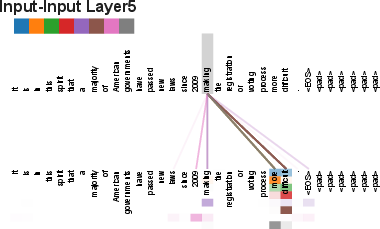
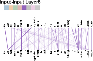
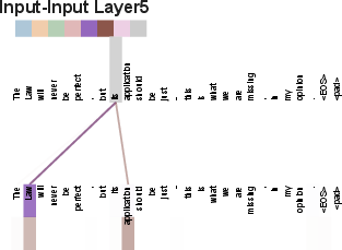
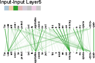
- Multi-head attention: Parallel attention mechanisms that project queries, keys, and values into multiple subspaces to capture diverse relations. "Multi-head attention allows the model to jointly attend to information from different representation subspaces at different positions."
- Penn Treebank: A widely used annotated corpus of English text with syntactic parses. "We trained a 4-layer transformer with on the Wall Street Journal (WSJ) portion of the Penn Treebank \citep{marcus1993building}, about 40K training sentences."
- Perplexity: A measure of LLM uncertainty; lower values indicate better predictive performance. "This hurts perplexity, as the model learns to be more unsure, but improves accuracy and BLEU score."
- Positional encodings: Deterministic or learned vectors added to token embeddings to inject sequence order information. "To this end, we add 'positional encodings' to the input embeddings at the bottoms of the encoder and decoder stacks."
- Residual connection: A skip connection that adds the input of a sub-layer to its output to ease optimization of deep networks. "We employ a residual connection \citep{he2016deep} around each of the two sub-layers, followed by layer normalization"
- Restricted self-attention: Self-attention constrained to a local window to reduce complexity for very long sequences. "self-attention could be restricted to considering only a neighborhood of size in the input sequence centered around the respective output position."
- Scaled Dot-Product Attention: An attention mechanism that scales query–key dot products by before softmax to stabilize gradients. "We call our particular attention 'Scaled Dot-Product Attention' (Figure~\ref{fig:multi-head-att})."
- Self-attention: An attention mechanism that relates positions within the same sequence to compute context-aware representations. "Self-attention, sometimes called intra-attention is an attention mechanism relating different positions of a single sequence in order to compute a representation of the sequence."
- Separable convolutions: Factorized convolutions that reduce computational cost by separating spatial and channel-wise processing. "Separable convolutions \citep{xception2016}, however, decrease the complexity considerably, to ."
- Softmax: A normalization function that converts a vector of logits into a probability distribution. "apply a softmax function to obtain the weights on the values."
- Tensor2Tensor: A software library and repository of deep learning models and datasets used in the paper’s experiments. "The code we used to train and evaluate our models is available at \url{https://github.com/tensorflow/tensor2tensor}."
- Warmup steps: An initial training phase where the learning rate increases linearly before decaying, to stabilize optimization. "We used ."
- Word-piece: A subword vocabulary construction method often used in neural machine translation. "split tokens into a 32000 word-piece vocabulary \citep{wu2016google}."
- WMT: The Workshop on Machine Translation benchmark suite used to evaluate translation systems. "On the WMT 2014 English-to-German translation task, the big transformer model (Transformer (big) in Table~\ref{tab:wmt-results}) outperforms the best previously reported models (including ensembles) by more than $2.0$ BLEU"
- WSJ: The Wall Street Journal section of the Penn Treebank commonly used for parsing benchmarks. "We trained a 4-layer transformer with on the Wall Street Journal (WSJ) portion of the Penn Treebank \citep{marcus1993building}, about 40K training sentences."
Collections
Sign up for free to add this paper to one or more collections.