- The paper presents a theoretical analysis showing that weight decay combined with learning rate schedules causes a rapid spike in gradient norms near the end of training.
- Empirical results on ResNet-50 and large language models confirm that interactions with normalization layers destabilize the gradient-to-weight norm ratio.
- A modified weight decay strategy in the Adam optimizer, named AdamC, effectively stabilizes training dynamics and improves model convergence.
Why Gradients Rapidly Increase Near the End of Training
This essay explores the paper “Why Gradients Rapidly Increase Near the End of Training” which investigates the unexpected behavior of gradient norm increases during long-duration training runs of large machine learning models. The authors provide insights into the interaction between weight decay, normalization layers, and learning rate schedules leading to this behavior, and propose a method to correct it.
Gradient Norm Increase Phenomenon
During extensive training programs for LLMs, it is observed that gradient norms tend to increase sharply towards the end of the training process. This behavior, which has not been addressed in existing literature, results from the interplay between weight decay and learning rate schedules in models employing normalization layers such as LayerNorm or BatchNorm. The paper provides a detailed theoretical analysis of why the gradient norm increases and suggests a corrective approach to mitigate this issue.
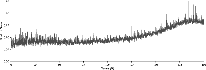
Figure 1: A 120M parameter LLM training run on FineWeb-Edu, showing the behavior where the gradient norm more than doubles towards the end of training.
Influence of Weight Decay, Normalization, and Learning Rate Schedules
The authors utilize theoretical frameworks to show that weight decay directly impacts the gradient-to-weight norm ratio during training. Specifically, the unintended side-effect is that altering the learning rate influences this ratio, which subsequently causes the gradient norm to increase undesirably.
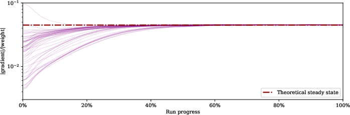
Figure 2: Gradient-to-weight ratios converge towards a steady equilibrium when training without a learning rate schedule.
To demonstrate this, the paper presents empirical results using image classification tasks on ImageNet with ResNet-50 models, showing that the gradient-to-weight norm ratios do converge towards a steady-state when a flat learning rate is used. However, when a cosine learning rate schedule is used, these ratios change over time, influenced by the schedule.
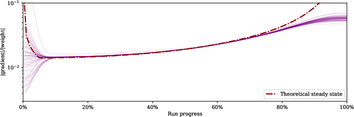
Figure 3: When a cosine learning rate schedule is used, the gradient-to-weight ratios are affected by the schedule.
Proposed Solution: Correcting Weight Decay
To address the aforementioned gradient norm increase, the paper proposes a modification to the weight decay algorithm that compensates for the variability caused by learning rate schedules. This modification recalibrates the balance of the weight norm relative to the gradient norm, keeping the changes consistent despite fluctuations in learning rates.
The adjusted method, dubbed AdamC (Corrected Adam), adapts the weight decay application according to the maximum learning rate used during the training schedule, effectively decoupling weight decay from learning rate adjustments. This ensures a stable gradient-to-weight norm ratio and averts the problematic increase of gradient norms observed towards the end of training scenarios.
Algorithm for Correcting Weight Decay
Below is the pseudocode for implementing the proposed correction in the Adam optimizer:
1
2
3
4
5
6
7
8
9
10
11
12
13
14
15
16
17
|
def adam_with_corrected_weight_decay(x_initial, learning_rate_schedule, gamma_max, decay_lambda, beta1, beta2, epsilon):
    v, m = 0, 0
    for t in range(T):
        for l in range(L):
            g_t = compute_gradient(x[l], zeta[l])  # Assuming compute_gradient fetches minibatch gradients
            m = beta1 * m + (1 - beta1) * g_t
            v = beta2 * v + (1 - beta2) * (g_t ** 2)
            m_hat = m / (1 - beta1 ** t)
            v_hat = v / (1 - beta2 ** t)

            if is_normalized_layer(l):
                x[l] = x[l] - learning_rate_schedule[t] * m_hat / (v_hat ** 0.5 + epsilon) - \
                    (learning_rate_schedule[t] ** 2 / gamma_max * decay_lambda) * x[l]
            else:
                x[l] = x[l] - learning_rate_schedule[t] * m_hat / (v_hat ** 0.5 + epsilon) - \
                    learning_rate_schedule[t] * decay_lambda * x[l]
return x |
In this implementation, the corrective factor is only applied to the normalized layers, while other layers follow the conventional AdamW decay strategy.
Experimental Validation
Experiments confirm the efficacy of the proposed correction mechanism on both image classification tasks and LLM pre-training. The correction leads to a substantial stabilization of gradient norms, demonstrating improvements in loss values compared to using standard optimizers.
These results indicate that the correction helps ensure more consistent training dynamics, supporting better network convergence and preventing gradient norm instability typically observed in long-duration training runs under varying learning rate schedules.
Conclusion
The study addresses a crucial component of training dynamics for large models by effectively managing gradient norm increases. The results suggest that the proposed theoretical insights and corrective weight decay procedures play a significant role in enhancing model performance and stability. Future research could explore additional enhancements to refine neural network training methodologies, particularly under complex and dynamic optimization scenarios.

