- The paper introduces SLOT, a test-time adaptation method that optimizes outputs with a sample-specific parameter vector.
- It employs a two-phase approach with lightweight gradient updates to boost performance on tasks like GSM8K and GPQA.
- It achieves significant accuracy gains and proper format adherence with less than 8% extra latency over baseline models.
Sample-specific LLM Optimization at Test-time (SLOT): An Academic Overview
Introduction and Motivation
LLMs continue to exhibit rapid gains in zero- and few-shot reasoning, yet evidence indicates that their ability to follow complex, highly-specific instructions remains inconsistent, especially when the target prompt deviates from distributions typically encountered at pretraining or instruction-tuning time. To address the misalignment between static, globally-trained parameters and the needs of individual queries, "SLOT: Sample-specific LLM Optimization at Test-time" (2505.12392) introduces a test-time adaptation framework—SLOT—that performs lightweight, sample-specific optimization exclusively during inference.
This method falls within the paradigm of Test-Time Adaptation (TTA), which aims for dynamic adjustment of model behavior in response to deployment-time data. Unlike prior TTA approaches that often involve extensive compute or require auxiliary self-supervision/reward signals, SLOT proposes an efficient and scalable modification to LLM inference, yielding substantial gains on standard benchmarks with negligible computational cost.
SLOT Methodology
SLOT relies on two core innovations: (1) prompt-specific, lightweight adaptation using a sample-specific parameter vector δ, and (2) architectural placement of this adaptation at the output layer (immediately before the LM head), enabling efficient feature caching and decoupling from the main transformer parameters.
The pipeline consists of two sequential phases:
- Prompt Stage: For each test prompt, initialize a parameter vector δ∈R1×d (where d is the model's hidden size) to zero. Iterate a small number T of gradient updates (typically 3–5 steps, using AdamW and learning rate η≈0.01), optimizing the cross-entropy loss on the input prompt only. Critically, the transformer forward computations can be cached, as only the (linear) LM head requires recomputation during these updates.
- Generation Stage: Use the optimized δ to shift the hidden features prior to token generation. Specifically, for each subsequent forward pass, the model's hidden states H are modulated as H′=H+δ. This directly induces a logit shift, interpreted as a Logit Modulation Vector (LMV).
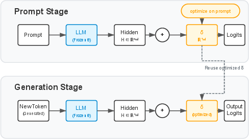
Figure 1: Overview of the SLOT pipeline, showing prompt-specific parameter optimization and subsequent re-use during autoregressive generation.
By broadcasting δ across sequence positions and reusing it per token, the method incurs only O(d) additional memory and requires no parameter updates to the main transformer, ensuring that adaptation is both instance-specific and non-destructive.
Empirical Results and Analysis
SLOT delivers consistent, significant improvements across diverse open LLMs (Qwen2.5, Llama-3.1, DeepSeek-R1-Distill variants) and tasks (arithmetic reasoning, math word problems, STEM Q&A, code generation, multilingual evaluations).
Notable quantitative findings include:
- GSM8K: Qwen2.5-7B with SLOT improves from 57.54% to 66.19% (+8.6%), with continuous gains as T increases from 0 to 5.
- GPQA: DeepSeek-R1-Distill-Llama-70B achieves 68.69%, marking a state-of-the-art performance among 70B-level open-source models.
SLOT demonstrates that with as few as three optimization steps, major improvements are realized, with diminishing returns for further steps. The computational overhead of optimization is marginal: on GSM8K with 5 iterations, inference latency increases by just 7.9% relative to the baseline.
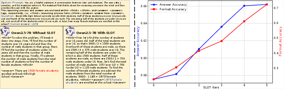
Figure 2: Left: An example where SLOT corrects both format and content errors in Qwen-2.5-7B's response. Right: GSM8K accuracy and answer-format compliance both climb with increasing SLOT iterations.
Error analyses and qualitative comparisons illustrate SLOT's effectiveness at recovering missed reasoning steps and adhering to prompt-specific formatting constraints.


Figure 3: Examples of original and SLOT-enhanced model responses on GSM8K; errors are resolved by test-time adaptation.
Ablation studies show that performance is robust across a broad range of learning rates and iteration counts, and that the method is insensitive to optimizer hyperparameters.
Mechanistic Insights
The LMV analysis reveals that SLOT systematically boosts the logits of reasoning-relevant tokens (e.g., reasoning',think’, step), promoting more faithful multi-step reasoning processes. Tokens corresponding to output endpoints (e.g., <|endoftext|>) and frequent content-neutral terms receive suppressed logits, delaying premature termination and emphasizing elaborate reasoning.
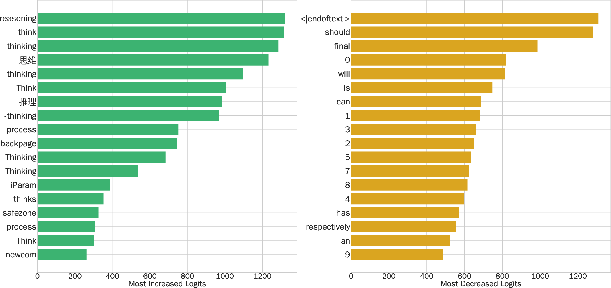
Figure 4: Most increased tokens under SLOT adaptation are linked to stepwise reasoning, while frequent numerals and modal verbs are discouraged.
The selective, instance-specific adjustment of model activations is thereby responsible for improved alignment with the intent and requirements of challenging prompts.
SLOT diverges markedly from in-context learning or parameter-efficient fine-tuning (PEFT) paradigms. PEFT techniques like LoRA, prompt-tuning, or prefix-tuning update a set of parameters that generalize across samples or tasks and are trained offline. By contrast, SLOT adapts on-the-fly, per-instance, and the adaptation is transient—δ is discarded after each sample is processed.
Test-Time Reinforcement Learning (TTRL) and extensive compute/majority-vote TTA strategies [li2025ttrl] do not offer the efficiency or simplicity of SLOT, as they require rollouts or complex reward modeling. Furthermore, SLOT incurs minimal risk of catastrophic forgetting or alignment drift, given the containment of adaptation to a lightweight vector and its operation at the interface layer.
Practical and Theoretical Implications
Practically, SLOT enables significant accuracy improvements on difficult reasoning and format-sensitive tasks with ultra-low inference cost, making it feasible to deploy in latency-sensitive or resource-constrained applications. The architectural design guarantees backwards compatibility with frozen, deployed models.
From a theoretical perspective, SLOT exposes the underfitting of LLMs to rare or unseen prompt structures, while demonstrating that much of this underfitting can be addressed by adjusting only the final activations. This reveals that a substantial portion of model incapacity on hard prompts is in fact addressable post-hoc, via minor additive modulation rather than deep retraining.
Additionally, the interpretability of the LMV provides insight into the tokenwise mechanisms underlying improved reasoning, supporting a line of research on the role of logit-level interventions in LLM behavior.
Potential Extensions and Future Work
Future lines of inquiry include:
- Extending SLOT to multimodal and cross-lingual LLMs;
- Adaptive strategies for choosing the number of test-time steps based on prompt complexity;
- Integrating instance-specific adaptation with dynamic retrieval or memory-augmented architectures;
- Employing more expressive adaptation schemes (e.g., low-rank adapters) while retaining efficiency guarantees.
There is also scope in exploring robust adaptation safeguards, especially in adversarial or fairness-sensitive deployments.
Conclusion
SLOT provides an efficient, test-time-only adaptation mechanism for LLMs, yielding substantial improvements in reasoning and format adherence by shifting a sample-specific activation vector at the output interface. Its efficacy across multiple architectures, benchmarks, and languages—coupled with negligible computational overhead and strong interpretability—positions SLOT as a robust method for practical post-hoc augmentation of foundation models.
Reference: "SLOT: Sample-specific LLM Optimization at Test-time" (2505.12392)

