Neural Networks with Physics-Informed Architectures and Constraints for Dynamical Systems Modeling

Abstract: Effective inclusion of physics-based knowledge into deep neural network models of dynamical systems can greatly improve data efficiency and generalization. Such a-priori knowledge might arise from physical principles (e.g., conservation laws) or from the system's design (e.g., the Jacobian matrix of a robot), even if large portions of the system dynamics remain unknown. We develop a framework to learn dynamics models from trajectory data while incorporating a-priori system knowledge as inductive bias. More specifically, the proposed framework uses physics-based side information to inform the structure of the neural network itself, and to place constraints on the values of the outputs and the internal states of the model. It represents the system's vector field as a composition of known and unknown functions, the latter of which are parametrized by neural networks. The physics-informed constraints are enforced via the augmented Lagrangian method during the model's training. We experimentally demonstrate the benefits of the proposed approach on a variety of dynamical systems -- including a benchmark suite of robotics environments featuring large state spaces, non-linear dynamics, external forces, contact forces, and control inputs. By exploiting a-priori system knowledge during training, the proposed approach learns to predict the system dynamics two orders of magnitude more accurately than a baseline approach that does not include prior knowledge, given the same training dataset.

• The paper introduces a framework that integrates known physics with neural networks, achieving an order-of-magnitude test loss reduction in system identification.
• It employs a compositional structure that combines physics-based functions with NN-parametrized unknowns and leverages differentiable ODE solvers for end-to-end training.
• Empirical results on systems such as the double pendulum and robotic simulators demonstrate robust extrapolation and significant constraint violation reduction via augmented Lagrangian optimization.

Physics-Informed Neural Networks for Dynamical Systems Identification

The paper introduces a framework for integrating physics-informed inductive biases—via both architectural design and constraint enforcement—within neural network (NN) models for nonlinear, high-dimensional dynamical systems. Recognizing the limitations of purely data-driven models in settings with high system complexity, limited data, or partially known dynamics, the framework leverages any available a priori knowledge as a compositional structure over the system's vector field and as explicit constraints during model training. Here, I discuss the key methods, implementation approaches, and empirical results, and then address practical implications and prospects for the field.

---

Framework Overview and Architectural Methodology

The method models the vector field $h(x, u)$ of a continuous-time dynamical system $\dot{x} = h(x, u)$, with $x$ the system state and $u$ the control vector. The innovation is to express $h$ as a composition of known functional structure $F(\cdot)$ and unknown terms parameterized by NNs: $$\dot{x} = h(x, u) = F(x, u, g_1(\cdot),...,g_d(\cdot))$$ where the $g_i$ are neural networks capturing the unknown (or partially known) terms of the dynamics (e.g., actuation, contact, or friction forces). The integration over $h$ is performed using end-to-end differentiable ODE solvers compatible with JAX or similar autodiff frameworks.

Implementation strategy:

• Known physics (e.g., system mass matrices, known couplings, symmetries, kinematic relationships) is incorporated directly as $F(\cdot)$, dictating the computation graph or neural ODE layer structure.
• Each unknown $g_i$ is typically a fully connected multilayer perceptron (MLP) using ReLU activations, but the underlying architecture can be adapted according to the priors' nature.
• The differentiable ODE solver (e.g., Runge-Kutta or adjoint methods) enables backpropagation through time for scalable optimization.

This compositional modeling enables strong inductive bias: prior knowledge does not regularize the loss, but structurally constrains the hypothesis space to models that extend and refine the existing known physical structure.

(Figure 1)

Figure 1: Diagram of the physics-informed neural ODE modeling framework. Known physics structure (blue) composes with unknown NN terms (red); constraints (yellow) are enforced broadly in state space, not just on labeled data.

---

Constraint Enforcement via Augmented Lagrangian Optimization

A key departure from classical physics-informed training is in the enforcement of equality and/or inequality constraints, derived from physical principles, across both observed and unobserved regions of the state space. These constraints take the form

$$\begin{align*} c_i(x, u, \theta) = 0 \quad &\forall (x, u) \in C_{i} \ c_j(x, u, \theta) \leq 0 \quad &\forall (x, u) \in C_{j} \end{align*}$$

and are imposed at a set of collocation points $(x_k, u_k)$ sampled from $C_i,C_j$ (potentially, much larger than the labeled dataset).

Enforcement is via a stochastic variant of the augmented Lagrangian method:

• Each constraint at each collocation point maintains its own Lagrange multiplier; primal-dual updates proceed via alternating stochastic gradient descent steps for the NN parameters and multiplier updates, with penalty parameters increased as violations decrease.
• The loss is thus: $$L(\theta, \lambda, \rho) = J(\theta) + \sum_{i,k} \left[ \lambda_{i,k} c_i(x_k,u_k;\theta) + \frac{\rho}{2} c_i(x_k,u_k;\theta)^2 \right] + ...$$ where $J(\theta)$ is the supervised prediction loss.

Implementation is efficient, as only random minibatches of constraints are evaluated per SGD step; this scales to tens of thousands of collocation points and constraints, and the dual update is embarrassingly parallel.

---

Experimental Results and Empirical Findings

Double Pendulum

Strong prior knowledge (mass, geometry, nonlinear vector field structure) is integrated into the NN via $F(\cdot)$, and additional equality constraints (e.g., vector field symmetries) are enforced. When training on a single time series, architectural priors alone yield an order-of-magnitude lower test loss; adding symmetry constraints yields another order-of-magnitude improvement. Inequality and geometric constraints are also successfully enforced across unlabeled state regions.

(Figure 2)

Figure 2: Loss evolution for double pendulum; K1: compositional vector field with known structure; K2: addition of four symmetry constraints.

Rigid-Body Multibody Robotic Systems (Brax Suite)

Benchmarks include Ant, Fetch, Humanoid, Reacher, and UR5E environments—each with high-dimensional states ($n=78-143$ for complex robots), contact, friction, and actuation.

Three scenarios are benchmarked:

• Baseline: Pure NN vector field, no inductive bias.
• K1: Structure imposes $\dot{q}=v$, known from physics.
• K2: Structure further imposes known mass matrices and (for some cases) the Jacobian; unknown actuation, friction, or contact forces remain as neural networks.
• K3–K4: Full structure including contact force constraints (laws of friction, e.g., $\|F_\mathrm{tang}\| \leq \mu F_\mathrm{norm}$).

Empirical conclusions:

• With the same data splits, testing error is improved by up to two orders of magnitude using the full prior architecture and constraints; robust prediction is observed with as few as 5–10 trajectories for K2/K3, compared to hundreds for the baseline.
• Constraint violation loss (e.g., contact/faster constraints) drops by up to four orders of magnitude compared to unconstrained models—indicating the augmented Lagrangian approach finds feasible solutions consistent with the underlying physics, not just low-loss ones.

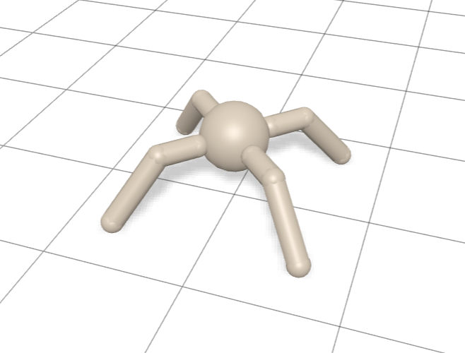
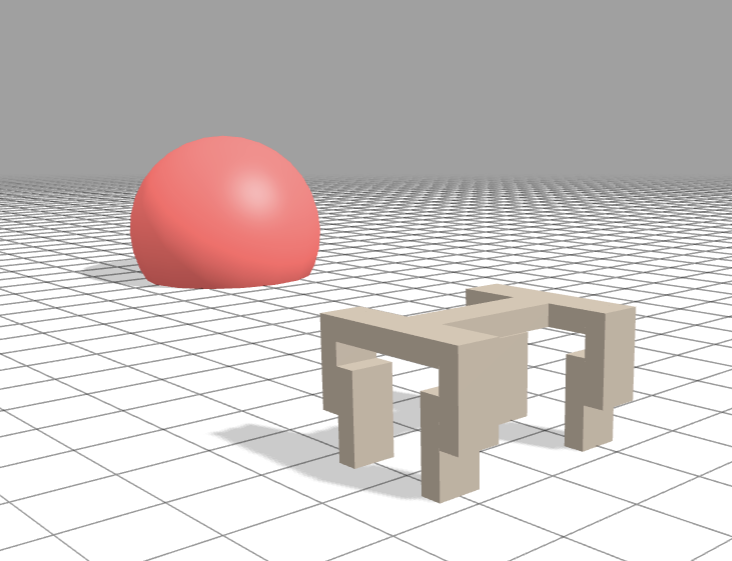
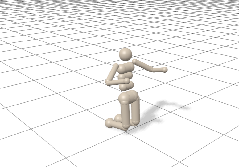
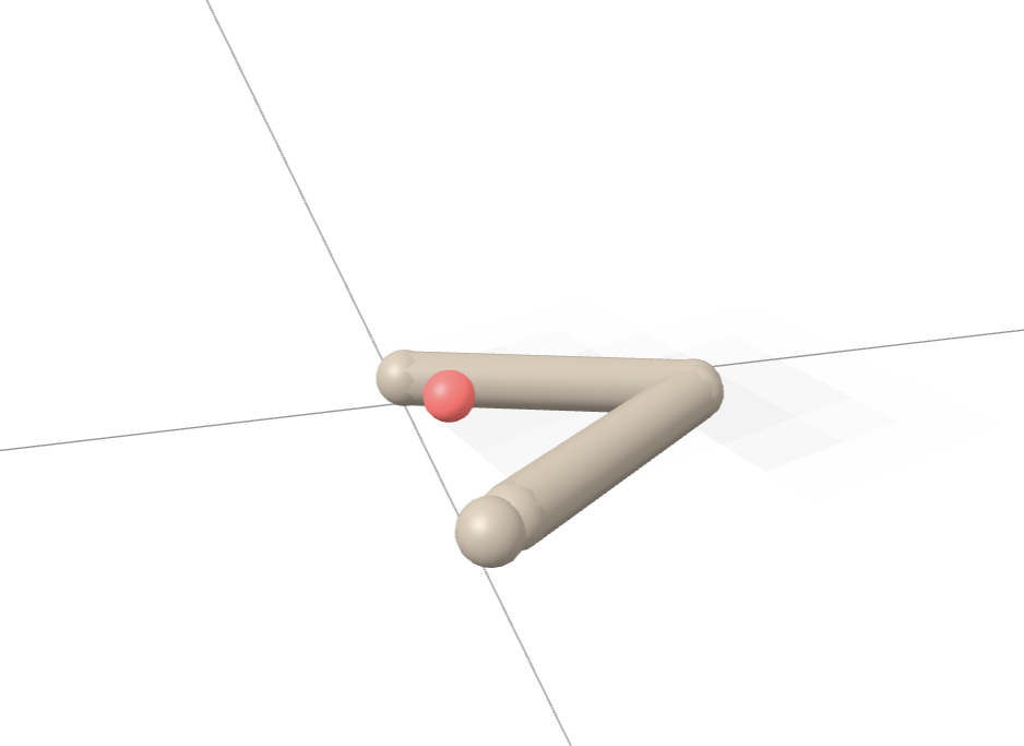
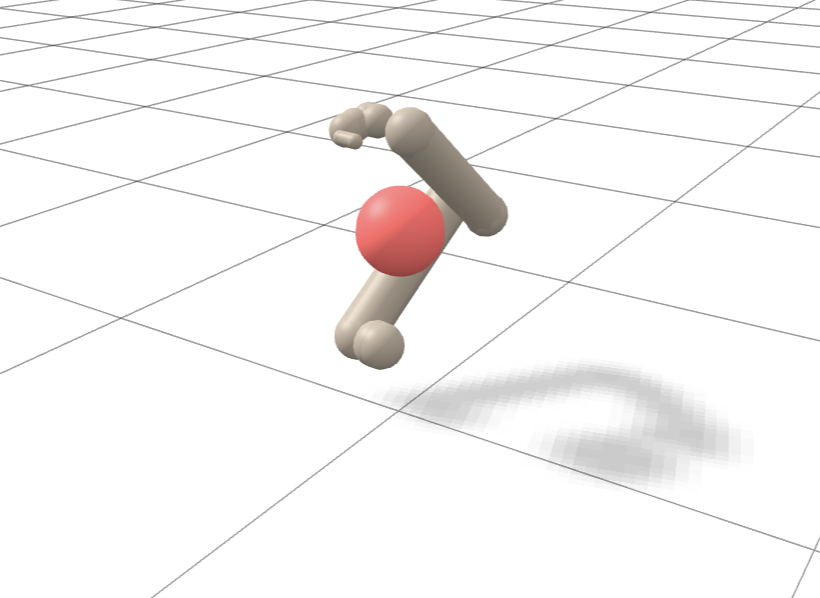
Figure 3: Illustration of the suite of simulated robotic systems used during testing.

---

Practical Implementation and Usage Recommendations

Key Choices

• ODE Integrator: Use adaptive-step solvers compatible with modern autodiff frameworks (e.g., JAX, PyTorch, or TensorFlow with SciPy or custom adjoint methods).
• Batching: Efficient implementation requires collocation constraint batching and, for very large system/state-action spaces, sharding constraint minibatches across hardware (multi-GPU/TPU).
• Parameterization: For known mechanical structures, mass/inertia, and kinematics, always code these in custom differentiable $F(\cdot)$ modules; only parameterize what is actually unknown, or what cannot be efficiently represented via analytic formulas.
• Constraint Mining: Inequality constraints (energy, dissipativity, friction, symmetries) greatly improve sample efficiency and out-of-distribution generalization even if they cannot be encoded in the architecture; sample collocation points broadly and check/expand constraint sets in a semi-supervised fashion.

Pitfalls

• Instability: If collocation points are poorly sampled, constraint satisfaction can be uneven across the state space. Uniform or stratified random sampling, plus progressive densification in high-violation regions, is recommended.
• Overfitting: For data-starved regimes, explicit architecture regularization and early stopping should be used in addition to the physics constraints.

---

Performance and Scaling Considerations

• Computational Cost: Augmented Lagrangian with batched constraints is tractable for batch sizes $>10^4$ per epoch; memory is dominated by saving Lagrange multipliers and constraint minibatch gradients.
• Scalability: Demonstrated on systems up to $n=143$ states (Fetch/Humanoid) and $m=10-17$ controls; scale is limited in practice by ODE solver forward+backward accumulation and memory bandwidth for constraint collocation.
• Generality: The method is agnostic to the specific choice of neural parameterization or optimizer, and it extends cleanly to hybrid and piecewise-smooth systems where known fragments of the vector field can be composed and unknown transitions parameterized by NNs.

---

Implications and Future Research Prospects

This work sets a new practical standard for physics-constrained system identification with NNs. In practice:

• It enables data-efficient learning for systems where partial physics knowledge is present (e.g., robot hardware, vehicle models, energetic priors).
• It yields not only improved interpolation but dramatically better extrapolation into unseen states—validated by out-of-distribution rollout error analysis.
• It provides a general recipe for bridging physical and empirical modeling: start with maximal physics-based structure, reserve NN learning to unknowns, and enforce any physics-based invariants or inequalities via scalable constrained stochastic optimization.

Limitations and next steps:

• The current approach requires careful constraint subsampling and may not optimally trade off constraint satisfaction and predictive accuracy outside the sampled set.
• Hybrid system transitions, non-smooth events (e.g., impacts), and discrete stochastic noise are not discussed; integrating these remains an open problem.
• Automated or active selection of collocation points for constraint enforcement, particularly in unexplored regions with high prediction uncertainty, would further increase robustness.

In broader context, this framework expands the toolbox for reliable, data-efficient modeling in domains where system identification from scratch is infeasible or cost-prohibitive—especially in real-world robotics, scientific computing, and safety-critical cyber-physical systems.

---

Conclusion

Physics-informed NNs with both architectural constraints and explicit, large-scale collocation constraint enforcement set a new bar for practical, scalable, and robust nonlinear system identification. As machine learning is increasingly integrated with physical modeling, this compositional and constrained approach balances theoretical guarantees with empirical flexibility, providing a promising path for reliable control, simulation, and planning in real-world high-dimensional systems.