- The paper introduces a generative neural architecture that integrates VAE for spatial compression and MDN-RNN for temporal prediction to build a robust world model.
- It demonstrates high performance in environments like CarRacing-v0 and VizDoom, showing effective policy learning and sim-to-real transfer.
- Results imply that compact, unsupervised world models can efficiently capture and predict complex dynamics, paving the way for scalable reinforcement learning applications.
World Models: A Detailed Summary
The paper "World Models" (1803.10122) investigates the generation of predictive models using neural networks for reinforcement learning (RL) environments, emphasizing unsupervised learning of spatial and temporal representations to create compact policies. By leveraging virtual environments generated by learned models, the policy can be trained in simulated scenarios and later deployed into real ones, enhancing practical applications of RL.
Introduction and Motivation
The authors draw a parallel between cognitive systems and artificial agents, proposing that understanding and predicting environmental dynamics enhances decision-making capabilities. Inspired by this, the architecture combines three components: Vision, Memory, and Controller. This architecture allows the model to compress and predict observations, enabling a simpler Controller to focus on decision making (Figure 1).
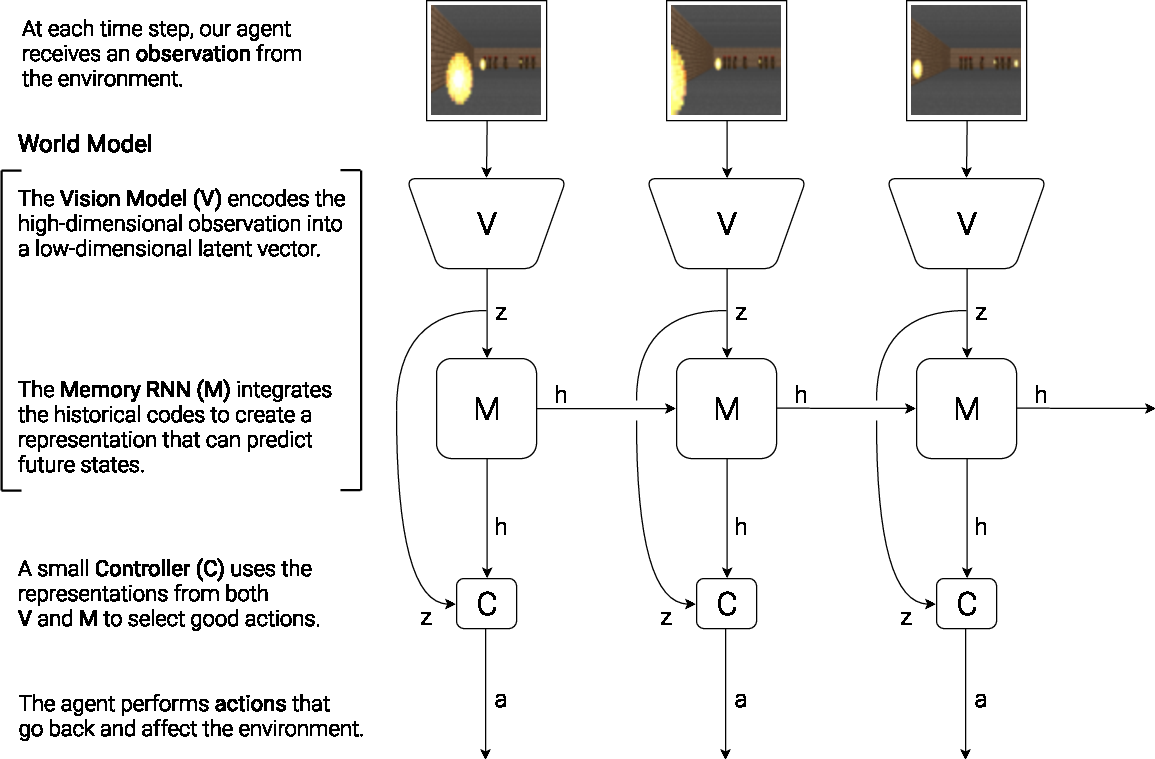
Figure 1: Our agent consists of three components that work closely together: Vision (V), Memory (M), and Controller (C).
Components of the World Model
VAE (Vision Model)
The Variational Autoencoder (VAE) is designed to compress observed high-dimensional inputs, such as video frames, into a latent space. This serves as the representation feeding other models without losing contextual understanding (Figure 2). The VAE is optimized for task-independent unsupervised learning to ensure its modularity across different scenarios.
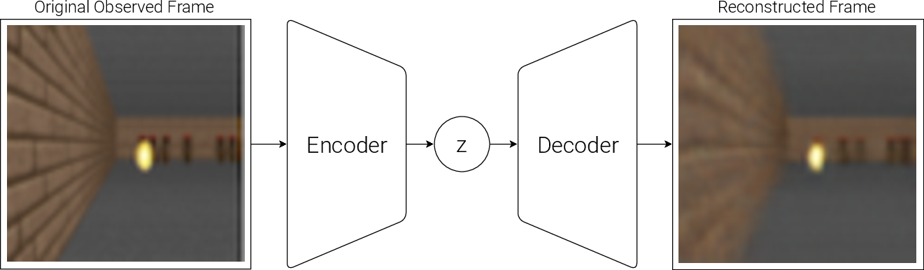
Figure 2: Flow diagram of a Variational Autoencoder (VAE).
MDN-RNN (Memory Model)
Positioned to handle temporal dynamics, the MDN-RNN captures sequential dependencies and predicts future states using a probabilistic approach. Unlike traditional deterministic models, it outputs distribution parameters allowing stochastic predictions crucial for uncertainty management (Figure 3).
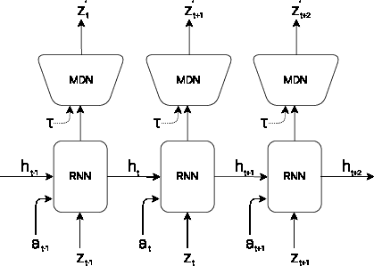
Figure 3: RNN with a Mixture Density Network output layer. The MDN outputs the parameters of a mixture of Gaussian distribution used to sample a prediction of the next latent vector z.
Controller Model
The Controller utilizes outputs from Vision and Memory to decide actions, designed to be lightweight for efficient training. It operates as a linear model, relying on evolution strategies for optimization rather than conventional backpropagation constrained by the credit assignment problem.
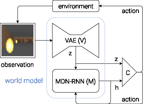
Figure 4: Flow diagram of our Agent model. The raw observation is first processed by V at each time step t to produce zt. The input into C is this latent vector zt concatenated with M's hidden state ht at each time step. C will then output an action vector at for motor control, and will affect the environment. M will then take the current zt and action at as an input to update its own hidden state to produce ht+1 to be used at time t+1.
Experiments and Results
Car Racing Experiment
In the CarRacing-v0 environment, the world model is trained using a dataset collected from random rollouts to derive a robust representation independent of performance bias (Figure 5). The resultant policy achieved scores well above the threshold required for acceptable task performance, demonstrating the efficacy of the model-based approach compared to previous methods reliant on extensive data preprocessing or frame stacking.
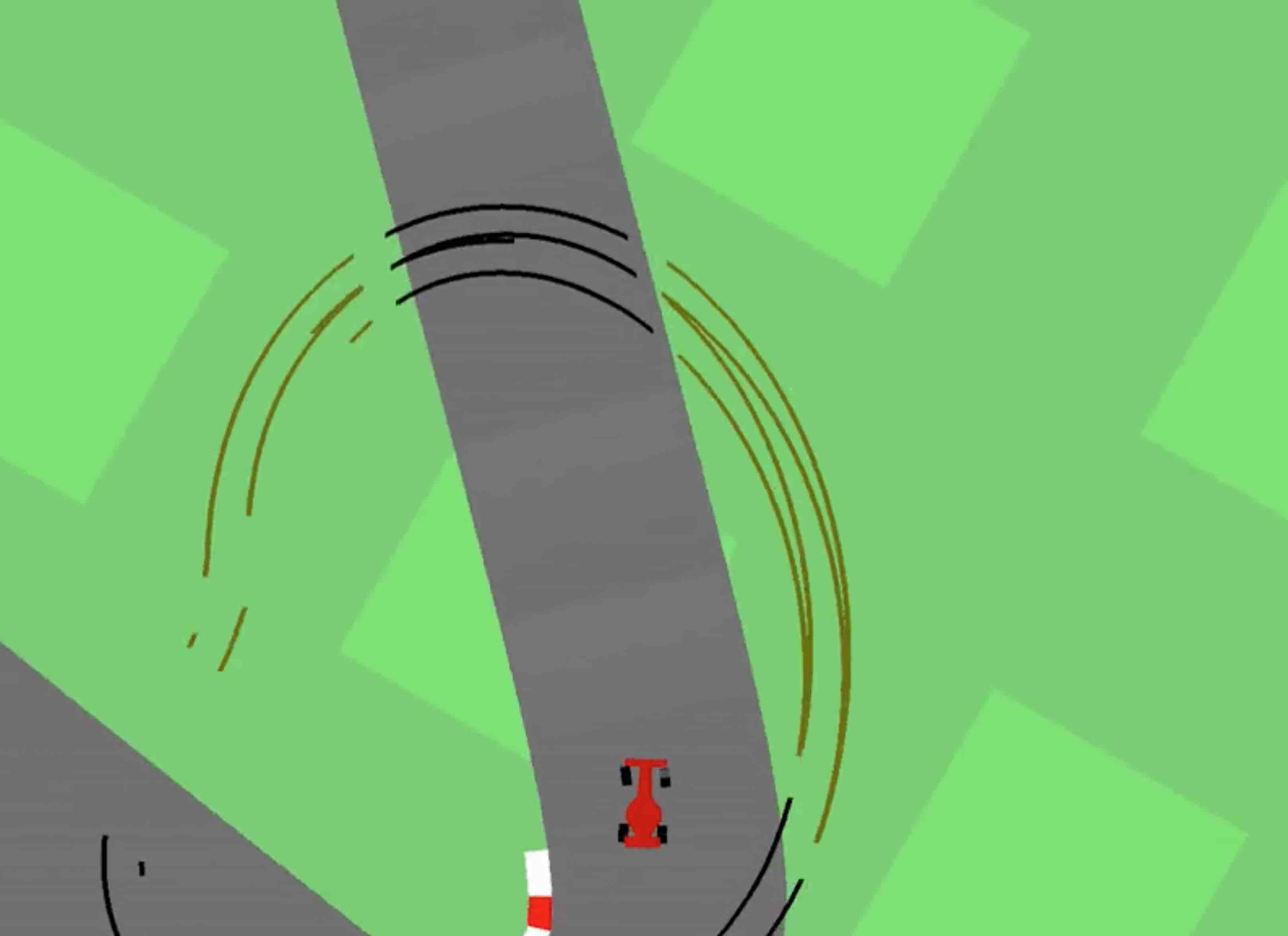
Figure 5: Our agent learning to navigate in CarRacing-v0.
VizDoom Experiment
The approach expanded to VizDoom's 'Take Cover' scenario demonstrating the feasibility of training entirely within a learned model environment. The agent transfers effectively between simulation and reality, achieving high survival scores (Figure 6). This suggests that the world model can generalize beyond simplistic environments, simulating complex interactions.
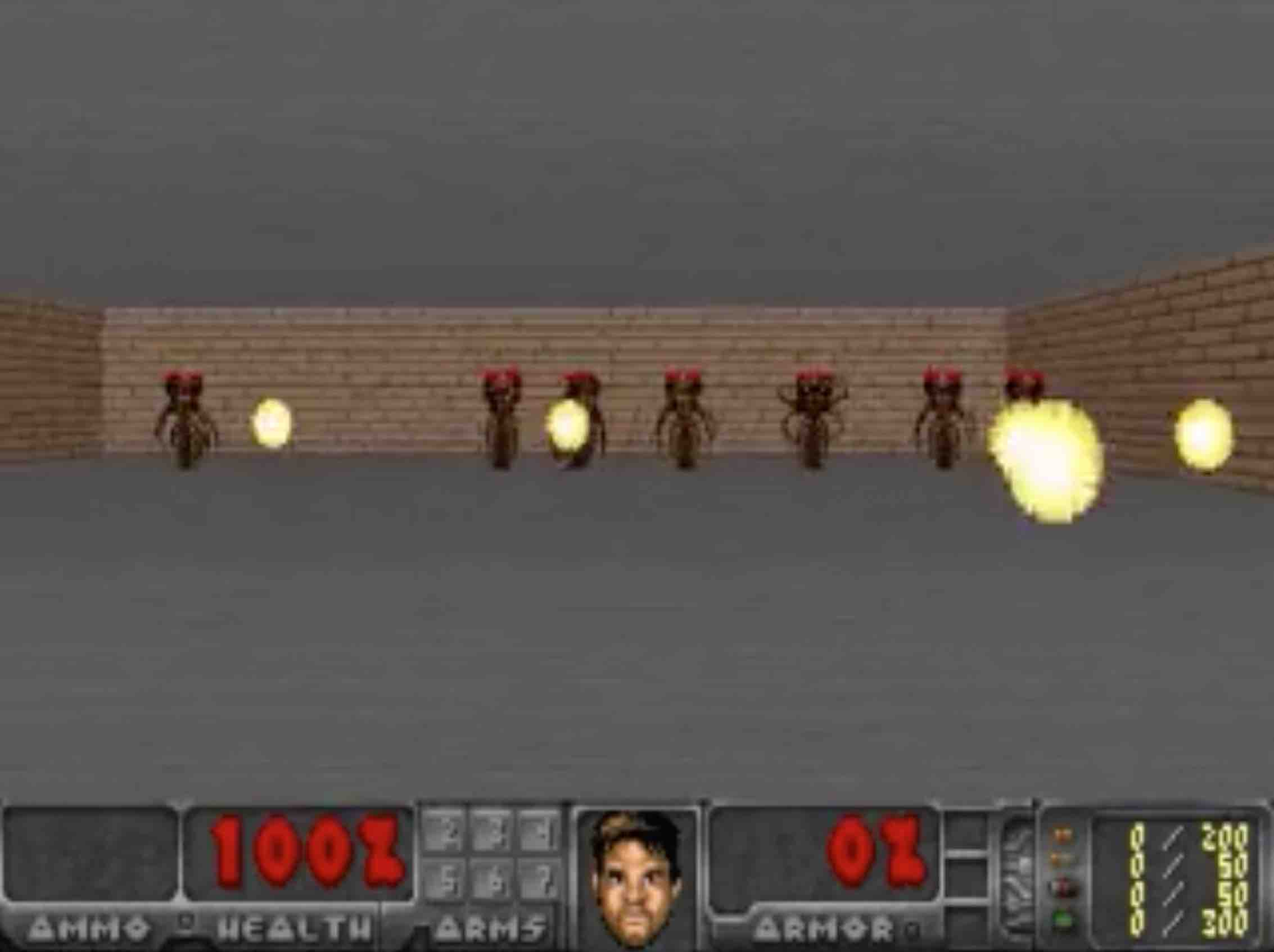
Figure 6: Our final agent solving VizDoom: Take Cover.
Implications and Future Directions
The research illustrates that compact yet expressive model-based approaches can compete with or surpass existing RL methods, particularly in scenarios where environment interaction is costly. It presents opportunities to incorporate curiosity-driven exploration and extend task applicability through iterative training. Future work could explore more complex hierarchical planning or incorporate advanced memory architectures to further emulate human cognitive capabilities.
Conclusion
"World Models" establishes a foundation for utilizing generative models in RL, showcasing task versatility and efficiency in agent policy learning. The model's ability to generalize via unsupervised learning components suggests significant potential for scaling in complexity while maintaining computational effectiveness, providing a promising direction for developing autonomous systems in the real world.
